Content from Before we Start

---

Last updated on 2026-02-19 | Edit this page

Introduction

---

Objective of the two days:

• No expeience required
• Information about R syntax, the RStudio interface, and move through how to import CSV files, the structure of data frames, how to add/remove rows and columns, how to calculate summary statistics from a data frame, and a brief introduction to plotting.

Overview

Questions

• How to find your way around RStudio?
• How to interact with R?
• How to manage your environment?
• How to install packages?

Objectives

• Install latest version of R.
• Install latest version of RStudio.
• Navigate the RStudio GUI.
• Install additional packages using the packages tab.
• Install additional packages using R code.

What is R? What is RStudio?

---

The term “R” is used to refer to both the programming language and the software that interprets the scripts written using it.

RStudio is currently a very popular way to not only write your R scripts but also to interact with the R software. To function correctly, RStudio needs R and therefore both need to be installed on your computer.

To make it easier to interact with R, we will use RStudio. RStudio is the most popular IDE (Integrated Development Environment) for R. An IDE is a piece of software that provides tools to make programming easier.

You can also use the R Presentations feature to present your work in an HTML5 presentation mixing Markdown and R code. You can display these within R Studio or your browser. There are many options for customising your presentation slides, including an option for showing LaTeX equations. This can help you collaborate with others and also has an application in teaching and classroom use. You can create application slides with the Shiny package, which allows you to create interactive web applications directly from R, reproducible document with R Markdown, and even interactive books with the bookdown package. Even create websites with the blogdown package. RStudio provides a great environment for all of these activities.

Why learn R?

---

R does not involve lots of pointing and clicking, and that’s a good thing

The learning curve might be steeper than with other software but with R, the results of your analysis do not rely on remembering a succession of pointing and clicking, but instead on a series of written commands, and that’s a good thing! So, if you want to redo your analysis because you collected more data, you don’t have to remember which button you clicked in which order to obtain your results; you just have to run your script again.

Working with scripts makes the steps you used in your analysis clear, and the code you write can be inspected by someone else who can give you feedback and spot mistakes.

Working with scripts forces you to have a deeper understanding of what you are doing, and facilitates your learning and comprehension of the methods you use.

R code is great for reproducibility

Reproducibility is when someone else (including your future self) can obtain the same results from the same dataset when using the same analysis.

R integrates with other tools to generate manuscripts from your code. If you collect more data, or fix a mistake in your dataset, the figures and the statistical tests in your manuscript are updated automatically.

An increasing number of journals and funding agencies expect analyses to be reproducible, so knowing R will give you an edge with these requirements.

To further support reproducibility and transparency, there are also packages that help you with dependency management: keeping track of which packages we are loading and how they depend on the package version you are using. This helps you make sure existing workflows work consistently and continue doing what they did before. We won’t be covering this in detail during the workshop.

R is interdisciplinary and extensible

With 10,000+ packages that can be installed to extend its capabilities, R provides a framework that allows you to combine statistical approaches from many scientific disciplines to best suit the analytical framework you need to analyze your data. For instance, R has packages for image analysis, GIS, time series, population genetics, and a lot more.

R works on data of all shapes and sizes

R is designed for data analysis. It comes with special data structures and data types that make handling of missing data and statistical factors convenient. Whether your dataset has hundreds or millions of lines, it won’t make much difference to you. R can connect to spreadsheets, databases, and many other data formats, on your computer or on the web.

R produces high-quality graphics

The plotting functionalities in R are endless, and allow you to adjust any aspect of your graph to convey most effectively the message from your data.

R has a large and welcoming community

Thousands of people use R daily. Many of them are willing to help you through mailing lists and websites such as Stack Overflow, or on the RStudio community. Questions which are backed up with short, reproducible code snippets are more likely to attract knowledgeable responses.

Not only is R free, but it is also open-source and cross-platform

Because R is open source and is supported by a large community of developers and users, there is a very large selection of third-party add-on packages which are freely available to extend R’s native capabilities.

RStudio extends what R can do, and makes it easier to write R code and interact with R. Left photo credit; Right photo credit.

Challenge

Exercise

Can you try to run R first then R studio and tell in the etherpad what differences you notice?

Show me the solution

You should see that R is a terminal-based interface, while RStudio is a graphical user interface (GUI) that provides additional tools and features to make working with R easier. RStudio has a more user-friendly interface with multiple panes for writing code, viewing plots, and managing files, while R is more basic and requires you to type commands directly into the terminal. We will explain what these panes and the terminal are and how to use them in the next section.

A tour of RStudio

---

Knowing your way around RStudio

---

Let’s start by learning about RStudio, which is an Integrated Development Environment (IDE) for working with R. It is open-source and free under the Affero General Public License (AGPL) v3.

We will use the RStudio IDE to write code, navigate the files on our computer, inspect the variables we create, and visualize the plots we generate. RStudio can also be used for other things (e.g., version control, developing packages, writing Shiny apps) that we will not cover during the workshop.

One of the advantages of using RStudio is that all the information you need to write code is available in a single window. Additionally, RStudio provides many shortcuts, autocompletion, and highlighting for the major file types you use while developing in R. RStudio makes typing easier and less error-prone.

Getting set up

---

It is good practice to keep a set of related data, analyses, and text self-contained in a single folder called the working directory. All of the scripts within this folder can then use relative paths to files. Relative paths indicate where inside the project a file is located (as opposed to absolute paths, which point to where a file is on a specific computer). Working this way makes it a lot easier to move your project around on your computer and share it with others without having to directly modify file paths in the individual scripts.

RStudio provides a helpful set of tools to do this through its “Projects” interface, which not only creates a working directory for you but also remembers its location (allowing you to quickly navigate to it). The interface also (optionally) preserves custom settings and open files to make it easier to resume work after a break.

Create a new project

• Under the File menu, click on New project, choose New directory, then New project
• Enter a name for this new folder (or “directory”) and choose a convenient location for it. This will be your working directory for the rest of the day (e.g., ~/data-carpentry)
• Click on Create project
• Create a new file where we will type our scripts. Go to File > New File > R script. Click the save icon on your toolbar and save your script as “script.R”.
• You should now have a file called script.R in your project directory.

The simplest way to open an RStudio project once it has been created is to navigate through your files to where the project was saved and double click on the .Rproj (blue cube) file. This will open RStudio and start your R session in the same directory as the .Rproj file. All your data, plots and scripts will now be relative to the project directory.

The RStudio Interface

Let’s take a quick tour of RStudio.

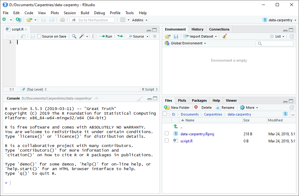
RStudio is divided into four “panes”. The placement of these panes and their content can be customized (see menu, Tools -> Global Options -> Pane Layout).

The Default Layout is:

• Top Left - Source: your scripts and documents
• Bottom Left - Console: what R would look and be like without RStudio
• Top Right - Environment/History: look here to see what you have done
• Bottom Right - Files and more: see the contents of the project/working directory here, like your Script.R file

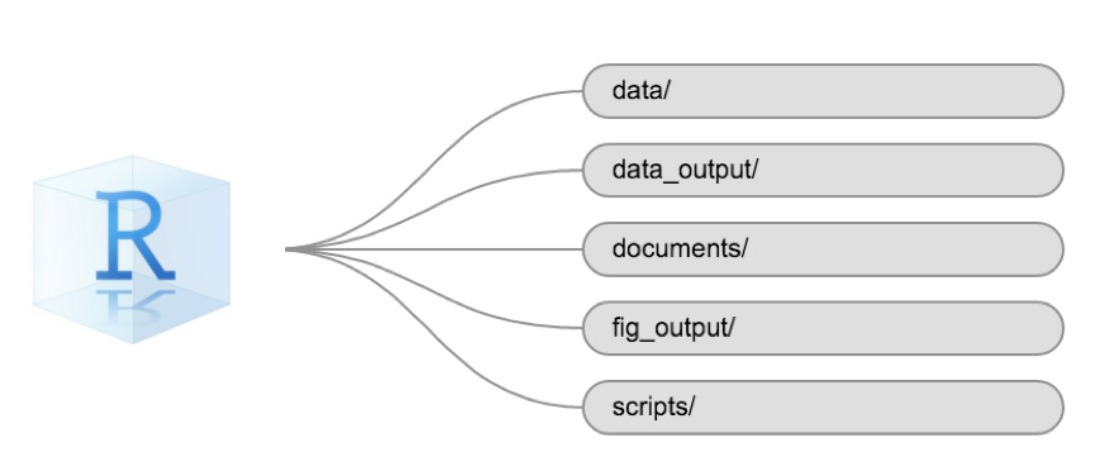
Organizing your working directory

Using a consistent folder structure across your projects will help keep things organized and make it easy to find/file things in the future. This can be especially helpful when you have multiple projects. In general, you might create directories (folders) for scripts, data, and documents. Here are some examples of suggested directories:

• data/ Use this folder to store your raw data and intermediate datasets. For the sake of transparency and provenance, you should always keep a copy of your raw data accessible and do as much of your data cleanup and preprocessing programmatically (i.e., with scripts, rather than manually) as possible.
• data_output/ When you need to modify your raw data, it might be useful to store the modified versions of the datasets in a different folder.
• documents/ Used for outlines, drafts, and other text.
• fig_output/ This folder can store the graphics that are generated by your scripts.
• scripts/ A place to keep your R scripts for different analyses or plotting.

You may want additional directories or subdirectories depending on your project needs, but these should form the backbone of your working directory.

The working directory

The working directory is an important concept to understand. It is the place where R will look for and save files. When you write code for your project, your scripts should refer to files in relation to the root of your working directory and only to files within this structure.

Using RStudio projects makes this easy and ensures that your working directory is set up properly.

If you need to check it, you can use getwd(). If for some reason your working directory is not the same as the location of your RStudio project, it is likely that you opened an R script or RMarkdown file not your .Rproj file. You should close out of RStudio and open the .Rproj file by double clicking on the blue cube!

If you ever need to modify your working directory in a script, setwd('my/path') changes the working directory. This should be used with caution since it makes analyses hard to share across devices and with other users.

Downloading the data and getting set up

For this lesson we will use the following folders in our working directory: data/, data_output/ and fig_output/. Let’s write them all in lowercase to be consistent. We can create them using the RStudio interface by clicking on the “New Folder” button in the file pane (bottom right), by creating them manually in your file explorer, or directly from R by typing at console:

R

dir.create("data")
dir.create("data_output")
dir.create("fig_output")

You can either download the data used for this lesson from GitHub or with R. You can copy the data from this GitHub link and paste it into a file called SAFI_clean.csv in the data/ directory you just created. Or you can do this directly from R by copying and pasting this in your terminal (your instructor can place this chunk of code in the Etherpad):

R

download.file(
  "https://raw.githubusercontent.com/datacarpentry/r-socialsci/main/episodes/data/SAFI_clean.csv",
  "data/SAFI_clean.csv", mode = "wb"
  )

Interacting with R

---

The basis of programming is that we write down instructions for the computer to follow, and then we tell the computer to follow those instructions. We write, or code, instructions in R because it is a common language that both the computer and we can understand. We call the instructions commands and we tell the computer to follow the instructions by executing (also called running) those commands.

There are two main ways of interacting with R: by using the console or by using script files (plain text files that contain your code). The console pane (in RStudio, the bottom left panel) is the place where commands written in the R language can be typed and executed immediately by the computer. It is also where the results will be shown for commands that have been executed. You can type commands directly into the console and press Enter to execute those commands, but they will be forgotten when you close the session.

Because we want our code and workflow to be reproducible, it is better to type the commands we want in the script editor and save the script. This way, there is a complete record of what we did, and anyone (including our future selves!) can easily replicate the results on their computer.

RStudio allows you to execute commands directly from the script editor by using the Ctrl + Enter shortcut (on Mac, Cmd + Return will work). The command on the current line in the script (indicated by the cursor) or all of the commands in selected text will be sent to the console and executed when you press Ctrl + Enter.

You can find other keyboard shortcuts in this RStudio cheatsheet about the RStudio IDE.

At some point in your analysis, you may want to check the content of a variable or the structure of an object without necessarily keeping a record of it in your script. You can type these commands and execute them directly in the console.

If R is ready to accept commands, the R console shows a > prompt. If R receives a command (by typing, copy-pasting, or sent from the script editor using Ctrl + Enter), R will try to execute it and, when ready, will show the results and come back with a new > prompt to wait for new commands.

If R is still waiting for you to enter more text, the console will show a + prompt. It means that you haven’t finished entering a complete command. This is likely because you have not ‘closed’ a parenthesis or quotation, i.e. you don’t have the same number of left-parentheses as right-parentheses or the same number of opening and closing quotation marks. When this happens, and you thought you finished typing your command, click inside the console window and press Esc; this will cancel the incomplete command and return you to the > prompt.

Installing additional packages using the packages tab

---

In addition to the core R installation, there are in excess of 10,000 additional packages which can be used to extend the functionality of R. Many of these have been written by R users and have been made available in central repositories, like the one hosted at CRAN, for anyone to download and install into their own R environment. You should have already installed the packages ‘ggplot2’ and ’dplyr. If you have not, please do so now using these instructions.

You can see if you have a package installed by looking in the packages tab (on the lower-right by default). You can also type the command installed.packages() into the console and examine the output.

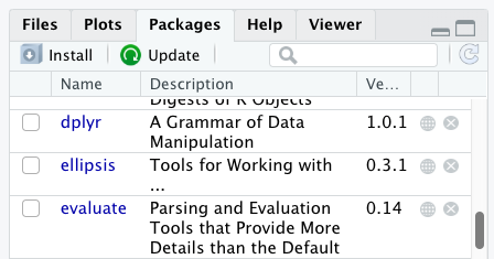
Additional packages can be installed from the ‘packages’ tab. On the packages tab, click the ‘Install’ icon and start typing the name of the package you want in the text box. As you type, packages matching your starting characters will be displayed in a drop-down list so that you can select them.

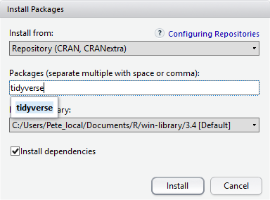
At the bottom of the Install Packages window is a check box to ‘Install’ dependencies. This is ticked by default, which is usually what you want. Packages can (and do) make use of functionality built into other packages, so for the functionality contained in the package you are installing to work properly, there may be other packages which have to be installed with them. The ‘Install dependencies’ option makes sure that this happens.

Challenge

Exercise

Use both the Console and the Packages tab to confirm that you have the tidyverse installed.

Show me the solution

Scroll through packages tab down to ‘tidyverse’. You can also type a few characters into the searchbox. The ‘tidyverse’ package is really a package of packages, including ‘ggplot2’ and ‘dplyr’, both of which require other packages to run correctly. All of these packages will be installed automatically. Depending on what packages have previously been installed in your R environment, the install of ‘tidyverse’ could be very quick or could take several minutes. As the install proceeds, messages relating to its progress will be written to the console. You will be able to see all of the packages which are actually being installed.

Because the install process accesses the CRAN repository, you will need an Internet connection to install packages.

Installing additional packages using R code

---

If you were watching the console window when you started the install of ‘tidyverse’, you may have noticed that the line

R

install.packages("tidyverse")

was written to the console before the start of the installation messages.

You could also have installed the tidyverse packages by running this command directly at the R terminal.

We will be using another package called here throughout the workshop to manage paths and directories. We will discuss it more detail in a later episode, but we will install it now in the console:

R

install.packages("here")

Key Points

• Use RStudio to write and run R programs.
• Use install.packages() to install packages (libraries).

Content from Introduction to R

---

Last updated on 2026-02-23 | Edit this page

Overview

Questions

• What data types are available in R?
• What is an object?
• How can objects of different data types be assigned to names?
• What arithmetic and logical operators can be used?
• How can subsets be extracted from vectors?
• How does R treat missing values?
• How can we deal with missing values in R?

Objectives

• Define the following terms as they relate to R: object, assign, call, function, arguments, options.
• Assign values to names in R.
• Learn how to name objects.
• Use comments to inform script.
• Solve simple arithmetic operations in R.
• Call functions and use arguments to change their default options.
• Inspect the content of vectors and manipulate their content.
• Subset values from vectors.
• Analyze vectors with missing data.

Creating objects in R

---

You can get output from R simply by typing math in the console:

R

3 + 5

OUTPUT

[1] 8

R

12 / 7

OUTPUT

[1] 1.714286

Everything that exists in R is an objects: from simple numerical values, to strings, to more complex objects like vectors, matrices, and lists. Even expressions and functions are objects in R.

However, to do useful and interesting things, we need to name objects. To do so, we need to give a name followed by the assignment operator <-, and the object we want to be named:

R

area_hectares <- 1.0

<- is the assignment operator. It assigns values (objects) on the right to names (also called symbols) on the left. So, after executing x <- 3, the value of x is 3. The arrow can be read as 3 goes into x. For historical reasons, you can also use = for assignments, but it is good practice to always use <- for assignments. More generally we prefer the <- syntax over = because it makes it clear what direction the assignment is operating (left assignment), and it increases the read-ability of the code.

In RStudio, typing Alt + - (push Alt at the same time as the - key) will write <- in a single keystroke in a PC, while typing Option + - (push Option at the same time as the - key) does the same in a Mac.

Objects can be given any name such as x, current_temperature, or subject_id. You want your object names to be explicit and not too long.

Objects’s name:

• cannot start with a number (2x is not valid, but x2 is).
• R is case sensitive (e.g., age is different from Age).
• There are some names that cannot be used because they are the names of fundamental objects in R (e.g.,if, else, for, see here for a complete list).
• It’s also best to avoid dots (.) within an object name as in my.dataset. There are many objects in R with dots in their names for historical reasons, but because dots have a special meaning in R (for methods) and other programming languages, it’s best to avoid them.
• The recommended writing style is called snake_case, which implies using only lowercaseletters and numbers and separating each word with underscores (e.g., animals_weight, average_income).
• It is also recommended to use nouns for object names, and verbs for function names.

It’s important to be consistent in the styling of your code (where you put spaces, how you name objects, etc.). Using a consistent coding style makes your code clearer to read for your future self and your collaborators.

Callout

Objects vs. variables

Depending on the context, name (of an object) and variable can have drastically different meanings. However, in this lesson, the two words are used synonymously.

When assigning an value to a name, R does not print anything. You can force R to print the value by using parentheses or by typing the object name:

R

area_hectares <- 1.0    # doesn't print anything
(area_hectares <- 1.0)  # putting parenthesis around the call prints the value of `area_hectares`

OUTPUT

[1] 1

R

area_hectares         # and so does typing the name of the object

OUTPUT

[1] 1

Now that R has area_hectares in memory, we can do arithmetic with it. For instance, we may want to convert this area into acres (area in acres is 2.47 times the area in hectares):

R

2.47 * area_hectares

OUTPUT

[1] 2.47

We can also change the value assigned to a name by assigning it a new one:

R

area_hectares <- 2.5
2.47 * area_hectares

OUTPUT

[1] 6.175

Assigning a value to one name does not change the values of other names. For example, let’s name the area in acres area_acres:

R

area_acres <- 2.47 * area_hectares

and then change (reassign) area_hectares to 50.

R

area_hectares <- 50

Challenge

Exercise

What do you think is the current value of area_acres? 123.5 or 6.175?

Show me the solution

The value of area_acres is still 6.175 because you have not re-run the line area_acres <- 2.47 * area_hectares since changing the value of area_hectares.

Comments

---

All programming languages allow the programmer to include comments in their code. Including comments to your code has many advantages: it helps you explain your reasoning and it forces you to be tidy. A commented code is also a great tool not only to your collaborators, but to your future self. Comments are the key to a reproducible analysis.

To do this in R we use the # character. Anything to the right of the # sign and up to the end of the line is treated as a comment and is ignored by R. You can start lines with comments or include them after any code on the line.

R

### This is a comment that starts the line. It is ignored by R.
area_hectares <- 1.0      # land area in hectares
area_acres <- area_hectares * 2.47  # convert to acres
area_acres        # print land area in acres.

OUTPUT

[1] 2.47

RStudio makes it easy to comment or uncomment a paragraph: after selecting the lines you want to comment, press at the same time on your keyboard Ctrl + Shift + C. If you only want to comment out one line, you can put the cursor at any location of that line (i.e. no need to select the whole line), then press Ctrl + Shift + C.

Challenge

Exercise

• Create two variables r_length and r_width and assign them values. It should be noted that, because length is a built-in R function, R Studio might add “()” after you type length and if you leave the parentheses you will get unexpected results. This is why you might see other programmers abbreviate common words.
• Create a third variable r_area and give it a value based on the current values of r_length and r_width.
• Show that changing the values of either r_length and r_width does not affect the value of r_area.
• What would you need to do to make sure that r_area always reflects the current values of r_length and r_width?

Show me the solution

R

r_length <- 2.5
r_width <- 3.2
r_area <- r_length * r_width
r_area

OUTPUT

[1] 8

R

# change the values of r_length and r_width
r_length <- 7.0
r_width <- 6.5
# the value of r_area isn't changed
r_area

OUTPUT

[1] 8

To make sure that r_area always reflects the current values of r_length and r_width, you would need to re-run the line r_area <- r_length * r_width after changing the values of r_length and r_width.

Functions and their arguments

• Functions are “scripts” that automate more complicated sets of commands including operations assignments, etc.
• Many functions are predefined, or can be made available by importing R packages (more on that later).
• A function usually gets one or more inputs called arguments.
• Functions often (but not always) return a value.

A typical example would be the function sqrt(). The input (the argument) must be a number, and the return value (in fact, the output) is the square root of that number. Executing a function (‘running it’) is called calling the function. An example of a function call is:

R

b <- sqrt(a)

Here, the value of a is given to the sqrt() function, the sqrt() function calculates the square root, and returns the value which is then assigned to the name b. This function is very simple, because it takes just one argument.

• The return ‘value’ of a function need not be numerical (like that of sqrt()), and it also does not need to be a single item: it can be a set of things, or even a dataset. We’ll see that when we read data files into R.
• Arguments can be anything, not only numbers or filenames, but also other objects.
• Exactly what each argument means differs per function, and must be looked up in the documentation (see below).
• Some functions take arguments which may either be specified by the user, or, if left out, take on a default value: these are called options. You can specify a value of your choice which will be used instead of the default.

Let’s try a function that can take multiple arguments: round().

R

round(3.14159)

OUTPUT

[1] 3

Here, we’ve called round() with just one argument, 3.14159, and it has returned the value 3. That’s because the default is to round to the nearest whole number. If we want more digits we can see how to do that by getting information about the round function. We can use args(round) or look at the help for this function using ?round.

R

args(round)

OUTPUT

function (x, digits = 0, ...)
NULL

R

?round

We see that if we want a different number of digits, we can type digits=2 or however many we want. We can also see the default value for digits is 0, which is why we got a whole number when we didn’t specify it.

R

round(3.14159, digits = 2)

OUTPUT

[1] 3.14

If you provide the arguments in the exact same order as they are defined you don’t have to name them:

R

round(3.14159, 2)

OUTPUT

[1] 3.14

And if you do name the arguments, you can switch their order:

R

round(digits = 2, x = 3.14159)

OUTPUT

[1] 3.14

It’s good practice to put the non-optional arguments (like the number you’re rounding) first in your function call, and to specify the names of all optional arguments. If you don’t, someone reading your code might have to look up the definition of a function with unfamiliar arguments to understand what you’re doing.

Discussion

Exercise

Type in ?round at the console and then look at the output in the Help pane. What other functions exist that are similar to round?

Vectors and data types

---

A vector is the most common and basic data type in R. A vector is composed by a series of values, which can be either numbers or characters. We can assign a series of values to a vector using the c() function. For example we can create a vector of the number of household members for the households we’ve interviewed and assign it to hh_members:

R

hh_members <- c(3, 7, 10, 6)
hh_members

OUTPUT

[1]  3  7 10  6

A vector can also contain characters. For example, we can have a vector of the building material used to construct our interview respondents’ walls (respondent_wall_type):

R

respondent_wall_type <- c("muddaub", "burntbricks", "sunbricks")
respondent_wall_type

OUTPUT

[1] "muddaub"     "burntbricks" "sunbricks"  

The quotes around “muddaub”, etc. are essential here. Without the quotes R will assume there are objects called muddaub, burntbricks and sunbricks. As these names don’t exist in R’s memory, there will be an error message.

R

respondent_wall_type <- c(muddaub, "burntbricks", "sunbricks")

ERROR

Error:
! object 'muddaub' not found

There are many functions that allow you to inspect the content of a vector. length() tells you how many elements are in a particular vector:

R

length(hh_members)

OUTPUT

[1] 4

R

length(respondent_wall_type)

OUTPUT

[1] 3

An important feature of a vector, is that all of the elements are the same type of data. The function typeof() indicates the type of an object:

R

typeof(hh_members)

OUTPUT

[1] "double"

R

typeof(respondent_wall_type)

OUTPUT

[1] "character"

The function str() provides an overview of the structure of an object and its elements. It is a useful function when working with large and complex objects:

R

str(hh_members)

OUTPUT

 num [1:4] 3 7 10 6

R

str(respondent_wall_type)

OUTPUT

 chr [1:3] "muddaub" "burntbricks" "sunbricks"

You can use the c() function to add other elements to your vector:

R

possessions <- c("bicycle", "radio", "television")
possessions <- c(possessions, "mobile_phone") # add to the end of the vector
possessions <- c("car", possessions) # add to the beginning of the vector
possessions

OUTPUT

[1] "car"          "bicycle"      "radio"        "television"   "mobile_phone"

In the first line, we take the original vector possessions, add the value "mobile_phone" to the end of it, and save the result back into possessions. Then we add the value "car" to the beginning, again saving the result back into possessions.

We can do this over and over again to grow a vector, or assemble a dataset. As we program, this may be useful to add results that we are collecting or calculating.

An atomic vector is the simplest R data type and is a linear vector of a single type. Above, we saw 2 of the 6 main atomic vector types that R uses: "character" and "numeric" (or "double"). These are the basic building blocks that all R objects are built from. The other 4 atomic vector types are:

• "logical" for TRUE and FALSE (the boolean data type)
• "integer" for integer numbers (e.g., 2L, the L indicates to R that it’s an integer)
• "complex" to represent complex numbers with real and imaginary parts (e.g., 1 + 4i) and that’s all we’re going to say about them
• "raw" for bitstreams that we won’t discuss further

Vectors are one of the many data structures that R uses. Other important ones are: + lists (list), + matrices (matrix), + data frames (data.frame), + factors (factor) + and arrays (array).

Challenge

Exercise

We’ve seen that atomic vectors can be of type character, numeric (or double), integer, and logical. But what happens if we try to mix these types in a single vector?

Show me the solution

R implicitly converts them to all be the same type.

Challenge

Exercise (continued)

What will happen in each of these examples? (hint: use class() to check the data type of your objects):

R

num_char <- c(1, 2, 3, "a")
num_logical <- c(1, 2, 3, TRUE)
char_logical <- c("a", "b", "c", TRUE)
tricky <- c(1, 2, 3, "4")

Why do you think it happens?

Show me the solution

Vectors can be of only one data type. R tries to convert (coerce) the content of this vector to find a “common denominator” that doesn’t lose any information.

Challenge

Exercise (continued)

How many values in combined_logical are "TRUE" (as a character) in the following example:

R

num_logical <- c(1, 2, 3, TRUE)
char_logical <- c("a", "b", "c", TRUE)
combined_logical <- c(num_logical, char_logical)

Show me the solution

Only one. There is no memory of past data types, and the coercion happens the first time the vector is evaluated. Therefore, the TRUE in num_logical gets converted into a 1 before it gets converted into "1" in combined_logical.

Discussion

Exercise (continued)

You’ve probably noticed that objects of different types get converted into a single, shared type within a vector. In R, we call converting objects from one class into another class coercion. These conversions happen according to a hierarchy, whereby some types get preferentially coerced into other types. Can you draw a diagram that represents the hierarchy of how these data types are coerced? (Optional)

Subsetting vectors

---

Subsetting (sometimes referred to as extracting or indexing) involves accessing out one or more values based on their numeric placement or “index” within a vector. If we want to subset one or several values from a vector, we must provide one index or several indices in square brackets. For instance:

R

respondent_wall_type <- c("muddaub", "burntbricks", "sunbricks")
respondent_wall_type[2]

OUTPUT

[1] "burntbricks"

R

respondent_wall_type[c(3, 2)]

OUTPUT

[1] "sunbricks"   "burntbricks"

We can also repeat the indices to create an object with more elements than the original one:

R

more_respondent_wall_type <- respondent_wall_type[c(1, 2, 3, 2, 1, 3)]
more_respondent_wall_type

OUTPUT

[1] "muddaub"     "burntbricks" "sunbricks"   "burntbricks" "muddaub"
[6] "sunbricks"  

R indices start at 1. Programming languages like Fortran, MATLAB, Julia, and R start counting at 1, because that’s what human beings typically do. Languages in the C family (including C++, Java, Perl, and Python) count from 0 because that’s simpler for computers to do.

Conditional subsetting

Another common way of subsetting is by using a logical vector. TRUE will select the element with the same index, while FALSE will not:

R

hh_members <- c(3, 7, 10, 6)
hh_members[c(TRUE, FALSE, TRUE, TRUE)]

OUTPUT

[1]  3 10  6

Typically, these logical vectors are not typed by hand, but are the output of other functions or logical tests. For instance, if you wanted to select only the values above 5:

R

hh_members > 5    # will return logicals with TRUE for the indices that meet the condition

OUTPUT

[1] FALSE  TRUE  TRUE  TRUE

R

## so we can use this to select only the values above 5
hh_members[hh_members > 5]

OUTPUT

[1]  7 10  6

You can combine multiple tests using & (both conditions are true, AND) or | (at least one of the conditions is true, OR):

R

hh_members[hh_members < 4 | hh_members > 7]

OUTPUT

[1]  3 10

R

hh_members[hh_members >= 4 & hh_members <= 7]

OUTPUT

[1] 7 6

• < stands for “less than”,
• > for “greater than”,
• >= for “greater than or equal to”,
• == for “equal to”. The double equal sign == is a test for numerical equality between the left and right hand sides, and should not be confused with the single = sign, which performs variable assignment (similar to <-).

A common task is to search for certain strings in a vector. One could use the “or” operator | to test for equality to multiple values, but this can quickly become tedious.

R

possessions <- c("car", "bicycle", "radio", "television", "mobile_phone")
possessions[possessions == "car" | possessions == "bicycle"] # returns both car and bicycle

OUTPUT

[1] "car"     "bicycle"

The function %in% allows you to test if any of the elements of a search vector (on the left hand side) are found in the target vector (on the right hand side):

R

possessions %in% c("car", "bicycle")

OUTPUT

[1]  TRUE  TRUE FALSE FALSE FALSE

R

c("car", "bicycle") %in% possessions

OUTPUT

[1] TRUE TRUE

Note that the output is the same length as the search vector on the left hand side, because %in% checks whether each element of the search vector is found somewhere in the target vector. Thus, you can use %in% to select the elements in the search vector that appear in your target vector:

R

possessions %in% c("car", "bicycle", "motorcycle", "truck", "boat", "bus")

OUTPUT

[1]  TRUE  TRUE FALSE FALSE FALSE

R

possessions[possessions %in% c("car", "bicycle", "motorcycle", "truck", "boat", "bus")]

OUTPUT

[1] "car"     "bicycle"

Missing data

---

As R was designed to analyze datasets, it includes the concept of missing data (which is uncommon in other programming languages). Missing data are represented in vectors as NA.

When doing operations on numbers, most functions will return NA if the data you are working with include missing values. This feature makes it harder to overlook the cases where you are dealing with missing data. You can add the argument na.rm=TRUE to calculate the result while ignoring the missing values.

R

rooms <- c(2, 1, 1, NA, 7)
mean(rooms)

OUTPUT

[1] NA

R

max(rooms)

OUTPUT

[1] NA

R

mean(rooms, na.rm = TRUE)

OUTPUT

[1] 2.75

R

max(rooms, na.rm = TRUE)

OUTPUT

[1] 7

If your data include missing values, you may want to become familiar with the functions is.na() and complete.cases(). See below for examples.

R

## Extract those elements which are not missing values.
## The ! character is also called the NOT operator
rooms[!is.na(rooms)]

OUTPUT

[1] 2 1 1 7

R

## Count the number of missing values.
## The output of is.na() is a logical vector (TRUE/FALSE equivalent to 1/0) so the sum() function here is effectively counting
sum(is.na(rooms))

OUTPUT

[1] 1

R

## Extract those elements which are complete cases. The returned object is an atomic vector of type `"numeric"` (or `"double"`).
rooms[complete.cases(rooms)]

OUTPUT

[1] 2 1 1 7

Recall that you can use the typeof() function to find the type of your atomic vector.

Challenge

Exercise

1. Using this vector of rooms, create a new vector with the NAs removed.

R

rooms <- c(1, 2, 1, 1, NA, 3, 1, 3, 2, 1, 1, 8, 3, 1, NA, 1)

2. Use the function median() to calculate the median of the rooms vector.

3. Use R to figure out how many households in the set use more than 2 rooms for sleeping.

Show me the solution

R

rooms <- c(1, 2, 1, 1, NA, 3, 1, 3, 2, 1, 1, 8, 3, 1, NA, 1)
rooms_no_na <- rooms[!is.na(rooms)]
# or
rooms_no_na <- rooms[complete.cases(rooms)]
# 2.
median(rooms, na.rm = TRUE)

OUTPUT

[1] 1

R

# 3.
rooms_above_2 <- rooms_no_na[rooms_no_na > 2]
length(rooms_above_2)

OUTPUT

[1] 4

Now that we have learned how to write scripts, and the basics of R’s data structures, we are ready to start working with the SAFI dataset we have been using in the other lessons, and learn about data frames.

Getting help

---

As mentioned in the functions and their arguments section, you can use a question mark ? to know more about a function (for example, typing ?round).

However, there are several other ways that people often get help when they are stuck with their R code.

• Search the internet: paste the last line of your error message or “R” and a short description of what you want to do into your favorite search engine and you will usually find several examples where other people have encountered the same problem and came looking for help.
  • Stack Overflow can be particularly helpful for this: answers to questions are presented as a ranked thread ordered according to how useful other users found them to be. You can search using the [r] tag.
  • Take care: copying and pasting code written by somebody else is risky unless you understand exactly what it is doing!
• Ask somebody “in the real world”. If you have a colleague or friend with more expertise in R than you have, show them the problem you are having and ask them for help.
• Sometimes, the act of articulating your question can help you to identify what is going wrong. This is known as “rubber duck debugging” among programmers.

Generative AI

We recommend that you avoid getting help from generative AI during the workshop for several reasons:

1. For most problems you will encounter at this stage, help and answers can be found among the first results returned by searching the internet.
2. The foundational knowledge and skills you will learn in this lesson by writing and fixing your own programs are essential to be able to evaluate the correctness and safety of any code you receive from online help or a generative AI chatbot. If you choose to use these tools in the future, the expertise you gain from learning and practicing these fundamentals on your own will help you use them more effectively.
3. As you start out with programming, the mistakes you make will be the kinds that have also been made – and overcome! – by everybody else who learned to program before you. Since these mistakes and the questions you are likely to have at this stage are common, they are also better represented than other, more specialized problems and tasks in the data that was used to train generative AI tools. This means that a generative AI chatbot is more likely to produce accurate responses to questions that novices ask, which could give you a false impression of how reliable they will be when you are ready to do things that are more advanced.

Key Points

• Access individual values by location using [].
• Access arbitrary sets of data using [c(...)].
• Use logical operations and logical vectors to access subsets of data.

Content from intro to Quarto (Optional)

---

Last updated on 2026-02-24 | Edit this page

Overview

Questions

• What is Quarto?
• How can I integrate my R code with text and plots?
• How can I convert .qmd files to .html?

Objectives

• Create a .qmd document containing R code, text, and plots
• Create a YAML header to control output
• Understand basic syntax of Quarto and Markdown
• Customise code chunks to control formatting
• Use code chunks and in-line code to create dynamic, reproducible documents

Quarto

---

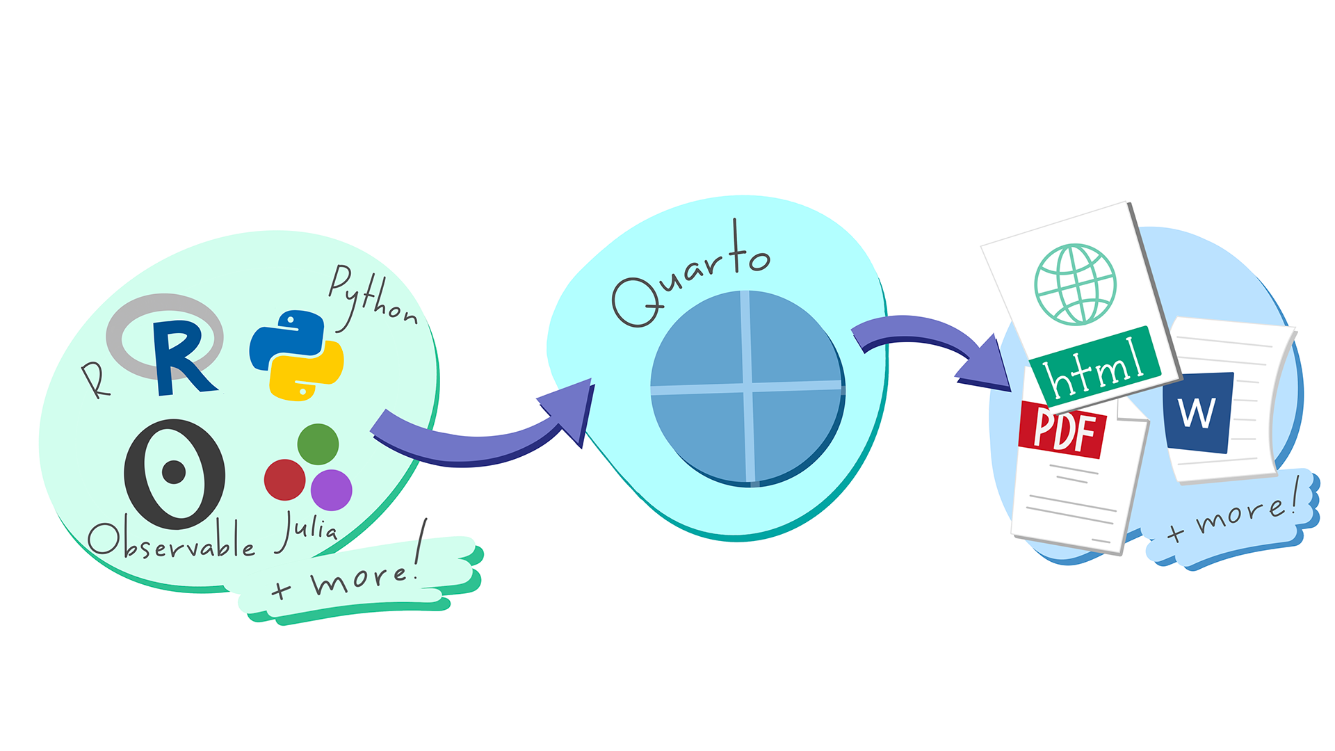
Quarto is a flexible type of document that allows you to seamlessly combine executable R code, and its output, with text in a single document. These documents can be readily converted to multiple static and dynamic output formats, including PDF (.pdf), Word (.docx), and HTML (.html).

The benefit of a well-prepared Quarto document is full reproducibility. This also means that, if you notice a data transcription error, or you are able to add more data to your analysis, you will be able to recompile the report without making any changes in the actual document.

Quarto comes pre-installed with RStudio (as of v2022.07), so no action is necessary.

A schematic representing the multi-language input **(e.g. Python, R Observable, Julia) and multi-format output (e.g. PDF, HTML, Word documents, and more) versatility of Quarto. Image source: Posit

Creating a Quarto file

---

To create a new Quarto document in RStudio, click File -> New File -> Quarto Document:

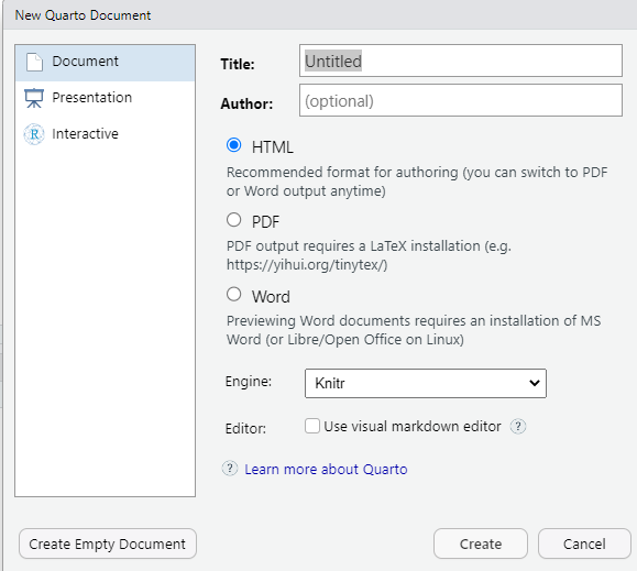
Then click on ‘Create Empty Document’. Normally you could enter the title of your document, your name (Author), and select the type of output, but we will be learning how to start from a blank document.

Basic components of Quarto

---

To control the output, a YAML (YAML Ain’t Markup Language) header is needed:

---
title: "My Awesome Report"
author: "Emmet Brickowski"
date: ""
format: html
---

The header is defined by the three hyphens at the beginning (---) and the three hyphens at the end (---).

Although not recommended, you can leave the YAML out. Then the output will be by default a HTML file. It’s still better to include the file format in the YAML header by adding the line format: html. You can also adapt the format of the file, to pdf or docx. We will start with an HTML document and discuss the other options later.

You can add more information about your document in the YAML header such as title, date and author. This information will be displayed at the top of your document. There are many more fields that can be added to the YAML header that provide additional information about the document or define the behaviour of the file. But we won’t discuss them now.

After the header, to begin the body of the document, you start typing after the end of the YAML header (i.e. after the second ---).

Markdown syntax

---

Markdown is a popular markup language that allows you to add formatting elements to text, such as bold, italics, and code. The formatting will not be immediately visible in a markdown (.md) document, like you would see in a Word document. Rather, you add Markdown syntax to the text, which can then be converted to various other files that can translate the Markdown syntax. Markdown is useful because it is lightweight, flexible, and platform independent.

Some platforms provide a real time preview of the formatting, like RStudio’s visual markdown editor (available from version 1.4).

First, let’s create a heading! A # in front of text indicates to Markdown that this text is a heading. Adding more #s make the heading smaller, i.e. one # is a first level heading, two ##s is a second level heading, etc. up to the 6th level heading.

# Title
## Section
### Sub-section
#### Sub-sub section
##### Sub-sub-sub section
###### Sub-sub-sub-sub section

(only use a level if the one above is also in use)

Since we have already defined our title in the YAML header, we will use a section heading to create an Introduction section.

## Introduction

You can make things bold by surrounding the word with double asterisks, **bold**, or double underscores, __bold__; and italicize using single asterisks, *italics*, or single underscores, _italics_.

You can also combine bold and italics to write something really important with triple-asterisks, ***really***, or underscores, ___really___; and, if you’re feeling bold (pun intended), you can also use a combination of asterisks and underscores, **_really_**, **_really_**. You can also use the keyboard shortcuts Ctrl+B for bold and Ctrl+I for italics on Windows and Linux, and Cmd+B for bold and Cmd+I for italics on Mac.

To create code-type font, surround the word with backticks, `code type`.

Now that we’ve learned a couple of things, it might be useful to implement them:

## Introduction

This report uses the **tidyverse** package along with the *SAFI* dataset,
which has columns that include:

Then we can create a list for the variables using -, +, or * keys.

## Introduction

This report uses the **tidyverse** package along with the *SAFI* dataset,
which has columns that include:

- village
- interview_date
- no_members
- years_liv
- respondent_wall_type
- rooms

You can also create an ordered list using numbers:

1. village
2. interview_date
3. no_members
4. years_liv
5. respondent_wall_type
6. rooms

And nested items by tab-indenting:

- village
  + Name of village
- interview_date
  + Date of interview
- no_members
  + How many family members lived in a house
- years_liv
  + How many years respondent has lived in village or neighbouring village
- respondent_wall_type
  + Type of wall of house
- rooms
  + Number of rooms in house

For more Markdown syntax see the following reference guide.

Now we can render the document into HTML by clicking the Render button in the top of the Source pane (top left), or use the keyboard shortcut Ctrl+Shift+K on Windows and Linux, and Cmd+Shift+K on Mac. If you haven’t saved the document yet, you will be prompted to do so when you Render for the first time.

Writing a Quarto report

---

Now we will add some R code from our previous data wrangling and visualisation, which means we need to make sure tidyverse is loaded. It is not enough to load tidyverse** from the console, we will need to load it within our Quarto document**. The same applies to our data. To load these, we will need to create a ‘code chunk’ at the top of our document (below the YAML header).

A code chunk can be inserted by clicking Code > Insert Chunk, or by using the keyboard shortcuts Ctrl+Alt+I on Windows and Linux, and Cmd+Option+I on Mac.

The syntax of a code chunk is:

MARKDOWN

```{r}
#| label: chunk-name
# Here is where you place the R code that you want to run.
```

A Quarto document knows that this text is not part of the report from the ``` that begins and ends the chunk. It also knows that the code inside of the chunk is R code from the r inside of the curly braces ({}). Below the curly braces, you can add code chunk options after the #| sign. In this way, you can for example add a label for the code chunk. Naming a chunk is optional, but recommended. Each chunk label must be unique, and only contain alphanumeric characters and -.

To load tidyverse and our SAFI_clean.csv file, we will insert a chunk and call it ‘setup’. Since we don’t want this code or the output to show in our rendered HTML document, we add an #| include: false option after the curly braces.

MARKDOWN

```{r}
#| label: setup
#| include: false
library(tidyverse)
library(here)
interviews <- read_csv(here("data/SAFI_clean.csv"), na = "NULL")
```

Callout

Important Note!

The file paths you give in a .qmd document, e.g. to load a .csv file, are relative to the .qmd document, not the project root.

As suggested in the Starting with Data episode, we highly recommend the use of the here() function to keep the file paths consistent within your project.

Customising chunk output

---

We mentioned using include: false in a code chunk to prevent the code and output from printing in the rendered document. There are additional options available to customise how the code-chunks are presented in the output document. The options are entered in the code chunk using the ‘hash pipe’, #|.

Option	Options	Output
eval	TRUE or FALSE	Whether or not the code within the code chunk should be run.
echo	TRUE or FALSE	Choose if you want to show your code chunk in the output document. echo = TRUE will show the code chunk.
include	TRUE or FALSE	Choose if the output of a code chunk should be included in the document. FALSE means that your code will run, but will not show up in the document.
warning	TRUE or FALSE	Whether or not you want your output document to display potential warning messages produced by your code.
message	TRUE or FALSE	Whether or not you want your output document to display potential messages produced by your code.
fig-align	default, left, right, center	Where the figure from your R code chunk should be output on the page

Callout

Tip

• The default settings for the above chunk options are all true.
• The default settings can be modified per chunk, or with knitr::opts_chunk$set(),
• Entering knitr::opts_chunk$set(echo = FALSE) will change the default of value of echo to FALSE for every code chunk in the document.

The defaults can also be changed in the YAML header with:

---
knitr:
  opts_chunk:
    echo: false
---

Insert table (self-directed learning)

---

Next, we will re-create a table from the Data Wrangling episode which shows the average household size grouped by village and memb_assoc. We can do this by creating a new code chunk and calling it ‘interview-tbl’. Or, you can come up with something more creative (just remember to stick to the naming rules).

It isn’t necessary to Render your document every time you want to see the output. Instead you can run the code chunk with the green triangle in the top right corner of the the chunk, or with the keyboard shortcuts: Ctrl+Alt+C on Windows and Linux, or Cmd+Option+C on Mac.

To make sure the table is formatted nicely in our output document, we will need to use the kable() function from the knitr package. The kable() function takes the output of your R code and renders it into a nice looking HTML table. You can also specify different aspects of the table, e.g. the column names, a caption, etc.

Load the data and the tidyverse package in a code chunk with include: false:

Run the code chunk to make sure you get the desired output.

R

interviews %>%
    filter(!is.na(memb_assoc)) %>%
    group_by(village, memb_assoc) %>%
    summarize(mean_no_membrs = mean(no_membrs)) %>%
  knitr::kable(col.names = c("Village", "Member Association", 
                             "Mean Number of Members"))

OUTPUT

`summarise()` has grouped output by 'village'. You can override using the
`.groups` argument.

Village	Member Association	Mean Number of Members
Chirodzo	no	8.062500
Chirodzo	yes	7.818182
God	no	7.133333
God	yes	8.000000
Ruaca	no	7.178571
Ruaca	yes	9.500000

When you are generating a table in quarto the label should be prefixed with tbl-, e.g. tbl-interviews. You can add a caption to the chunk options with tbl-cap: "Your caption here".

MARKDOWN

```{r}
#| label: tbl-interviews
#| tbl-cap: "A useful description about the table."
interviews %>%
    filter(!is.na(memb_assoc)) %>%
    group_by(village, memb_assoc) %>%
    summarize(mean_no_membrs = mean(no_membrs)) %>%
  knitr::kable(col.names = c("Village", "Member Association", 
                             "Mean Number of Members"))
```

OUTPUT

`summarise()` has grouped output by 'village'. You can override using the
`.groups` argument.

A useful description about the table.

Village	Member Association	Mean Number of Members
Chirodzo	no	8.062500
Chirodzo	yes	7.818182
God	no	7.133333
God	yes	8.000000
Ruaca	no	7.178571
Ruaca	yes	9.500000

Many different R packages can be used to generate tables. Some of the more commonly used options are listed in the table below.

Name	Creator(s)	Description
condformat	Oller Moreno (2022)	Apply and visualize conditional formatting to data frames in R. It renders a data frame with cells formatted according to criteria defined by rules, using a tidy evaluation syntax.
DT	Xie et al. (2023)	Data objects in R can be rendered as HTML tables using the JavaScript library ‘DataTables’ (typically via R Markdown or Shiny). The ‘DataTables’ library has been included in this R package.
formattable	Ren and Russell (2021)	Provides functions to create formattable vectors and data frames. ‘Formattable’ vectors are printed with text formatting, and formattable data frames are printed with multiple types of formatting in HTML to improve the readability of data presented in tabular form rendered on web pages.
flextable	Gohel and Skintzos (2023)	Use a grammar for creating and customizing pretty tables. The following formats are supported: ‘HTML’, ‘PDF’, ‘RTF’, ‘Microsoft Word’, ‘Microsoft PowerPoint’ and R ‘Grid Graphics’. ‘R Markdown’, ‘Quarto’, and the package ‘officer’ can be used to produce the result files.
gt	Iannone et al. (2022)	Build display tables from tabular data with an easy-to-use set of functions. With its progressive approach, we can construct display tables with cohesive table parts. Table values can be formatted using any of the included formatting functions.
huxtable	Hugh-Jones (2022)	Creates styled tables for data presentation. Export to HTML, LaTeX, RTF, ‘Word’, ‘Excel’, and ‘PowerPoint’. Simple, modern interface to manipulate borders, size, position, captions, colours, text styles and number formatting.
pander	Daróczi and Tsegelskyi (2022)	Contains some functions catching all messages, ‘stdout’ and other useful information while evaluating R code and other helpers to return user specified text elements (e.g., header, paragraph, table, image, lists etc.) in ‘pandoc’ markdown or several types of R objects similarly automatically transformed to markdown format.
pixiedust	Nutter and Kretch (2021)	‘pixiedust’ provides tidy data frames with a programming interface intended to be similar to ’ggplot2’s system of layers with fine-tuned control over each cell of the table.
reactable	Lin et al. (2023)	Interactive data tables for R, based on the ‘React Table’ JavaScript library. Provides an HTML widget that can be used in ‘R Markdown’ or ‘Quarto’ documents, ‘Shiny’ applications, or viewed from an R console.
rhandsontable	Owen et al. (2021)	An R interface to the ‘Handsontable’ JavaScript library, which is a minimalist Excel-like data grid editor.
stargazer	Hlavac (2022)	Produces LaTeX code, HTML/CSS code and ASCII text for well-formatted tables that hold regression analysis results from several models side-by-side, as well as summary statistics.
tables	Murdoch (2022)	Computes and displays complex tables of summary statistics. Output may be in LaTeX, HTML, plain text, or an R matrix for further processing.
tangram	Garbett et al. (2023)	Provides an extensible formula system to quickly and easily create production quality tables. The processing steps are a formula parser, statistical content generation from data defined by a formula, and rendering into a table.
xtable	Dahl et al. (2019)	Coerce data to LaTeX and HTML tables.
ztable	Moon (2021)	Makes zebra-striped tables (tables with alternating row colors) in LaTeX and HTML formats easily from a data.frame, matrix, lm, aov, anova, glm, coxph, nls, fitdistr, mytable and cbind.mytable objects.

Challenge

Exercise

Play around with the different options in the chunk with the code for the table, and re-Render to see what each option does to the output.

What happens if you use eval: false and echo: false? What is the difference between this and include: false?

Solution to Exercise

Create a chunk with eval: false, echo: false, then create another chunk with include: false to compare. eval: false and echo: false will neither run the code in the chunk, nor show the code in the rendered document. The code chunk essentially doesn’t exist in the rendered document as it was never run. Whereas include: false will run the code and store the output for later use.

In-line R code (self-directed learning)

---

Now we will use some in-line R code to present some descriptive statistics. To use in-line R-code, we use the same backticks that we used in the Markdown section, with an r to specify that we are generating R-code. The difference between in-line code and a code chunk is the number of backticks. In-line R code uses one backtick (r), whereas code chunks use three backticks (r).

For example, today’s date is `r Sys.Date()`, will be rendered as: today’s date is 2026-02-24.
The code will display today’s date in the output document (well, technically the date the document was last rendered).

The best way to use in-line R code, is to minimise the amount of code you need to produce the in-line output by preparing the output in code chunks. Let’s say we’re interested in presenting the average household size in a village.

R

# create a summary data frame with the mean household size by village
mean_household <- interviews %>%
    group_by(village) %>%
    summarize(mean_no_membrs = mean(no_membrs))

# and select the village we want to use
mean_chirodzo <- mean_household %>%
  filter(village == "Chirodzo")

Now we can make an informative statement on the means of each village, and include the mean values as in-line R-code. For example:

The average household size in the village of Chirodzo is `r round(mean_chirodzo$mean_no_membrs, 2)`

becomes…

The average household size in the village of Chirodzo is 7.08.

Because we are using in-line R code instead of the actual values, we have created a dynamic document that will automatically update if we make changes to the dataset and/or code chunks.

Plots (self-directed learning)

---

Finally, we will also include a plot, so our document is a little more colourful and a little less boring. We will use the interview_plotting data from the previous episode.

If you were unable to complete the previous lesson or did not save the data, then you can create it in a new code chunk.

R

## Not run, but can be used to load in data from previous lesson!
interviews_plotting <- interviews %>%
  ## pivot wider by items_owned
  separate_rows(items_owned, sep = ";") %>%
  ## if there were no items listed, changing NA to no_listed_items
  replace_na(list(items_owned = "no_listed_items")) %>%
  mutate(items_owned_logical = TRUE) %>%
  pivot_wider(names_from = items_owned, 
              values_from = items_owned_logical, 
              values_fill = list(items_owned_logical = FALSE)) %>%
  ## pivot wider by months_lack_food
  separate_rows(months_lack_food, sep = ";") %>%
  mutate(months_lack_food_logical = TRUE) %>%
  pivot_wider(names_from = months_lack_food, 
              values_from = months_lack_food_logical, 
              values_fill = list(months_lack_food_logical = FALSE)) %>%
  ## add some summary columns
  mutate(number_months_lack_food = rowSums(select(., Jan:May))) %>%
  mutate(number_items = rowSums(select(., bicycle:car)))

Plots created in Quarto should have a label prefixed with fig-, e.g. #| label: fig-fancy-plot.

Challenge

Exercise

Create a new code chunk for the plot, and copy the code from any of the plots we created in the previous episode to produce a plot in the chunk. I recommend one of the colourful plots.

If you are feeling adventurous, you can also create a new plot with the interviews_plotting data frame.

Solution to Exercise

MARKDOWN

```{r}
#| label: fig-fancy-plot
#| answer: true
#| purl: false
interviews_plotting %>%
  ggplot(aes(x = respondent_wall_type)) +
  geom_bar(aes(fill = village))
```

We can also create a caption with the chunk option fig-cap: "Caption here", and add some nicer labels using the labs() function.

MARKDOWN

```{r}
#| label: fig-chunk-name
#| fig-cap: "I made this plot while attending an awesome Data Carpentries workshop where I learned a ton of cool stuff!"
#| echo: false

interviews_plotting %>%
  ggplot(aes(x = respondent_wall_type)) +
  geom_bar(aes(fill = village), position = "dodge") + 
  labs(x = "Type of Wall in Home", y = "Count", fill = "Village Name") +
  scale_fill_viridis_d() # add colour deficient friendly palette
```

I made this plot while attending an awesome Data Carpentries workshop where I learned a ton of cool stuff!

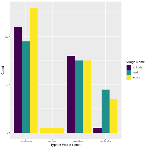
…or, ideally, something more informative.

Now, you may have been wondering why I insisted that you prefix the labels of your tables in figures, but there is a useful reason for this! It allows you to cross-reference them in the text of your document, and it requires that the label is unique, and that they have the correct prefix.

For example, we can talk about the table we made earlier and reference it using the label @tbl-interview, which, when rendered, becomes Table 1.

We can do the same with our figures. For example, @fig-fancy-plot becomes Figure 1. The number will of course depend on whether any plots or figures comes before it, but since you just need to reference the label, there’s no need to know what number a specific plot has in a document (especially useful for figure-heavy documents).

Other output options (self-directed learning)

---

You can convert Quarto to a PDF or a Word document (among others). Put pdf or word in the initial header of the file to indicate the desired output format.

---
format: word
---

Callout

Note: Creating PDF documents

Creating .pdf documents may require installation of some extra software. The R package tinytex provides some tools to help make this process easier for R users. With tinytex installed, run tinytex::install_tinytex() to install the required software (you’ll only need to do this once) and then when you render to pdf tinytex will automatically detect and install any additional LaTeX packages that are needed to produce the pdf document. Visit the tinytex website for more information.

Callout

Note: Inserting citations into a Quarto file

It is possible to insert citations into a Quarto file using the editor toolbar. The editor toolbar includes commonly seen formatting buttons generally seen in text editors (e.g., bold and italic buttons). The toolbar is accessible by using the settings dropdown menu (next to the ‘Render’ dropdown menu) to select ‘Use Visual Editor’, also accessible through the shortcut ‘Crtl+Shift+F4’. From here, clicking ‘Insert’ allows ‘Citation’ to be selected (shortcut: ‘Crtl+Shift+F8’). For example, searching ‘10.1007/978-3-319-24277-4’ in ‘From DOI’ and inserting will provide the citation for ggplot2 [@wickham2016]. This will also save the citation(s) in ‘references.bib’ in the current working directory.

Visit the R Studio website for more information. Tip: obtaining citation information from relevant packages can be done by using citation("package").

Resources

---

• Markdown tutorial
• Official Quarto website (comprehensive resource of tutorials and documentation)
• Welcome to Quarto - workshop by Posit (former RStudio)
• R Markdown: The Definitive Guide - book by the RStudio team on R Markdown, the predecessor of Quarto

Key Points

• Quarto is useful for creating reproducible documents combining text and executable R code.
• Specify chunk options to control formatting of the output document

Content from Starting with Data

---

Last updated on 2026-02-23 | Edit this page

Overview

Questions

• What is a data.frame?
• How can I read a complete csv file into R?
• How can I get basic summary information about my dataset?
• How can I change the way R treats strings in my dataset?
• Why would I want strings to be treated differently?

Objectives

• Describe what a data frame is.
• Load external data from a .csv file into a data frame.
• Summarize the contents of a data frame.
• Subset values from data frames.
• Change how character strings are handled in a data frame.

What are data frames?

---

• Data frames are the de facto data structure for tabular data in R, and what we use for data processing, statistics, and plotting.
• A data frame is the representation of data in the format of a table where the columns are vectors that all have the same length.
• Data frames are analogous to the more familiar spreadsheet in programs such as Excel, with one key difference.
• Because columns are vectors, each column must contain a single type of data (e.g., characters, integers, factors).

Data frames can be created by hand, but most commonly they are generated by the functions read_csv() or read_table(); in other words, when importing spreadsheets from your hard drive (or the web). We will now demonstrate how to import tabular data using read_csv().

Presentation of the SAFI Data

---

• SAFI (Studying African Farmer-Led Irrigation) is a study looking at farming and irrigation methods in Tanzania and Mozambique.

• The survey data was collected through interviews conducted between November 2016 and June 2017.

• For this lesson, we will be using a subset of the available data.

• For information about the full teaching dataset used in other lessons in this workshop, see the dataset description.

• We will be using a subset of the cleaned version of the dataset that was produced through cleaning in OpenRefine (data/SAFI_clean.csv).

• In this dataset, the missing data is encoded as “NULL”, each row holds information for a single interview respondent, and the columns represent:

column_name	description
key_id	Added to provide a unique Id for each observation. (The InstanceID field does this as well but it is not as convenient to use)
village	Village name
interview_date	Date of interview
no_membrs	How many members in the household?
years_liv	How many years have you been living in this village or neighboring village?
respondent_wall_type	What type of walls does their house have (from list)
rooms	How many rooms in the main house are used for sleeping?
memb_assoc	Are you a member of an irrigation association?
affect_conflicts	Have you been affected by conflicts with other irrigators in the area?
liv_count	Number of livestock owned.
items_owned	Which of the following items are owned by the household? (list)
no_meals	How many meals do people in your household normally eat in a day?
months_lack_food	Indicate which months, In the last 12 months have you faced a situation when you did not have enough food to feed the household?
instanceID	Unique identifier for the form data submission

Importing data

---

• You are going to load the data in R’s memory using the function read_csv() from the readr package, which is part of the tidyverse.
• readr gets installed as part as the tidyverse installation.
• When you load the tidyverse (library(tidyverse)), the core packages (the packages used in most data analyses) get loaded, including readr.

Before proceeding, however, this is a good opportunity to talk about conflicts.

• Certain packages we load can end up introducing function names that are already in use by pre-loaded R packages.
• For instance, when we load the tidyverse package below, we will introduce two conflicting functions: filter() and lag(). This happens because filter and lag are already functions used by the stats package (already pre-loaded in R).
• What will happen now is that if we, for example, call the filter() function, R will use the dplyr::filter() version and not the stats::filter() one. This happens because, if conflicted, by default R uses the function from the most recently loaded package.
• Conflicted functions may cause you some trouble in the future, so it is important that we are aware of them so that we can properly handle them, if we want.

To do so, we just need the following functions from the conflicted package:

• conflicted::conflict_scout(): Shows us any conflicted functions.
  
• conflict_prefer("function", "package_prefered"): Allows us to choose the default function we want from now on.
  
• It is also important to know that we can, at any time, just call the function directly from the package we want, such as stats::filter().

Path management

Even with the use of an RStudio project, it can be difficult to learn how to specify paths to file locations. The here package creates paths relative to the top-level directory (your RStudio project). These relative paths work regardless of where the associated source file lives inside your project, like analysis projects with data and reports in different subdirectories. This is an important contrast to using setwd(), which depends on the way you order your files on your computer.

Image credit: Allison Horst

• Before we can use the read_csv() and here() functions, we need to load the tidyverse and here packages.
• Also, if you recall, the missing data is encoded as “NULL” in the dataset. We’ll tell it to the function, so R will automatically convert all the “NULL” entries in the dataset into NA.

R

library(tidyverse)
library(here)

interviews <- read_csv(
  here("data", "SAFI_clean.csv"), 
  na = "NULL")

The following code snippets show how the path to the data file would be specified using setwd() and read.csv(), and how it is specified using here() and read_csv():

R

setwd("../data")
read.csv("SAFI_clean.csv")

• This works only if your working directory is scripts/ or source/.
  
• If you open the project with project.Rproj, your working directory is project/, so setwd("../data") will fail (there is no ../data from project/).

R

library(here)
read.csv(here("data", "SAFI_clean.csv"))

• This always works, no matter where the script is located or how you open the project.
• here() finds the project root (where project.Rproj is) and builds the path from there.
• Your code is portable and reproducible.

In the above code, we notice the here() function takes folder and file names as inputs (e.g., "data", "SAFI_clean.csv"), each enclosed in quotations ("") and separated by a comma. The here() will accept as many names as are necessary to navigate to a particular file (e.g., here("analysis", "data", "surveys", "clean", "SAFI_clean.csv)).

The here() function can accept the folder and file names in an alternate format, using a slash (“/”) rather than commas to separate the names. The two methods are equivalent, so that here("data", "SAFI_clean.csv") and here("data/SAFI_clean.csv") produce the same result. (The slash is used on all operating systems; backslashes are not used.)

If you were to type in the code above, it is likely that the read.csv() function would appear in the automatically populated list of functions. This function is different from the read_csv() function, as it is included in the “base” packages that come pre-installed with R. Overall, read.csv() behaves similar to read_csv(), with a few notable differences. First, read.csv() coerces column names with spaces and/or special characters to different names (e.g. interview date becomes interview.date). Second, read.csv() stores data as a data.frame, where read_csv() stores data as a different kind of data frame called a tibble. We prefer tibbles because they have nice printing properties among other desirable qualities. Read more about tibbles here.

• The second statement in the code above creates a data frame but doesn’t output any data because, as you might recall, assignments (<-) don’t display anything. (Note, however, that read_csv may show informational text about the data frame that is created.)
• If we want to check that our data has been loaded, we can see the contents of the data frame by typing its name: interviews in the console.

R

interviews
## Try also
## view(interviews)
## head(interviews)

OUTPUT

# A tibble: 131 × 14
   key_ID village  interview_date      no_membrs years_liv respondent_wall_type
    <dbl> <chr>    <dttm>                  <dbl>     <dbl> <chr>
 1      1 God      2016-11-17 00:00:00         3         4 muddaub
 2      2 God      2016-11-17 00:00:00         7         9 muddaub
 3      3 God      2016-11-17 00:00:00        10        15 burntbricks
 4      4 God      2016-11-17 00:00:00         7         6 burntbricks
 5      5 God      2016-11-17 00:00:00         7        40 burntbricks
 6      6 God      2016-11-17 00:00:00         3         3 muddaub
 7      7 God      2016-11-17 00:00:00         6        38 muddaub
 8      8 Chirodzo 2016-11-16 00:00:00        12        70 burntbricks
 9      9 Chirodzo 2016-11-16 00:00:00         8         6 burntbricks
10     10 Chirodzo 2016-12-16 00:00:00        12        23 burntbricks
# ℹ 121 more rows
# ℹ 8 more variables: rooms <dbl>, memb_assoc <chr>, affect_conflicts <chr>,
#   liv_count <dbl>, items_owned <chr>, no_meals <dbl>, months_lack_food <chr>,
#   instanceID <chr>

Callout

Note

• read_csv() assumes that fields are delimited by commas.
• However, in several countries, the comma is used as a decimal separator and the semicolon (;) is used as a field delimiter.
• If you want to read in this type of files in R, you can use the read_csv2 function. It behaves exactly like read_csv but uses different parameters for the decimal and the field separators. If you are working with another format, they can be both specified by the user. + Check out the help for read_csv() by typing ?read_csv to learn more.
• There is also the read_tsv() for tab-separated data files, and read_delim() allows you to specify more details about the structure of your file.

Note that read_csv() actually loads the data as a tibble. A tibble is an extension of R data frames used by the tidyverse. When the data is read using read_csv(), it is stored in an object of class tbl_df, tbl, and data.frame. You can see the class of an object with

R

class(interviews)

OUTPUT

[1] "spec_tbl_df" "tbl_df"      "tbl"         "data.frame" 

As a tibble, the type of data included in each column is listed in an abbreviated fashion below the column names. For instance, here key_ID is a column of floating point numbers (abbreviated <dbl> for the word ‘double’), village is a column of characters (<chr>) and the interview_date is a column in the “date and time” format (<dttm>).

Inspecting data frames

---

• When calling a tbl_df object (like interviews here), there is already a lot of information about our data frame being displayed such as the number of rows, the number of columns, the names of the columns, and as we just saw the class of data stored in each column.
• However, there are functions to extract this information from data frames. Here is a non-exhaustive list of some of these functions. Let’s try them out!

Size:

• dim(interviews) - returns a vector with the number of rows as the first element, and the number of columns as the second element (the dimensions of the object)
• nrow(interviews) - returns the number of rows
• ncol(interviews) - returns the number of columns

Content:

• head(interviews) - shows the first 6 rows
• tail(interviews) - shows the last 6 rows

Names:

• names(interviews) - returns the column names (synonym of colnames() for data.frame objects)

Summary:

• str(interviews) - structure of the object and information about the class, length and content of each column
• summary(interviews) - summary statistics for each column
• glimpse(interviews) - returns the number of columns and rows of the tibble, the names and class of each column, and previews as many values will fit on the screen. Unlike the other inspecting functions listed above, glimpse() is not a “base R” function so you need to have the dplyr or tibble packages loaded to be able to execute it.

Note: most of these functions are “generic.” They can be used on other types of objects besides data frames or tibbles.

Subsetting data frames

---

Our interviews data frame has rows and columns (it has 2 dimensions). In practice, we may not need the entire data frame; for instance, we may only be interested in a subset of the observations (the rows) or a particular set of variables (the columns). If we want to access some specific data from it, we need to specify the “coordinates” (i.e., indices) we want from it. Row numbers come first, followed by column numbers.

R

## first element in the first column of the tibble
interviews[1, 1]

OUTPUT

# A tibble: 1 × 1
  key_ID
   <dbl>
1      1

R

## first element in the 6th column of the tibble 
interviews[1, 6]

OUTPUT

# A tibble: 1 × 1
  respondent_wall_type
  <chr>
1 muddaub             

R

## first column of the tibble (as a vector)
interviews[[1]]

OUTPUT

  [1]   1   2   3   4   5   6   7   8   9  10  11  12  13  14  15  16  17  18
 [19]  19  20  21  22  23  24  25  26  27  28  29  30  31  32  33  34  35  36
 [37]  37  38  39  40  41  42  43  44  45  46  47  48  49  50  51  52  53  54
 [55]  55  56  57  58  59  60  61  62  63  64  65  66  67  68  69  70  71 127
 [73] 133 152 153 155 178 177 180 181 182 186 187 195 196 197 198 201 202  72
 [91]  73  76  83  85  89 101 103 102  78  80 104 105 106 109 110 113 118 125
[109] 119 115 108 116 117 144 143 150 159 160 165 166 167 174 175 189 191 192
[127] 126 193 194 199 200

R

## first column of the tibble
interviews[1]

OUTPUT

# A tibble: 131 × 1
   key_ID
    <dbl>
 1      1
 2      2
 3      3
 4      4
 5      5
 6      6
 7      7
 8      8
 9      9
10     10
# ℹ 121 more rows

R

## first three elements in the 7th column of the tibble
interviews[1:3, 7]

OUTPUT

# A tibble: 3 × 1
  rooms
  <dbl>
1     1
2     1
3     1

R

## the 3rd row of the tibble
interviews[3, ]

OUTPUT

# A tibble: 1 × 14
  key_ID village interview_date      no_membrs years_liv respondent_wall_type
   <dbl> <chr>   <dttm>                  <dbl>     <dbl> <chr>
1      3 God     2016-11-17 00:00:00        10        15 burntbricks
# ℹ 8 more variables: rooms <dbl>, memb_assoc <chr>, affect_conflicts <chr>,
#   liv_count <dbl>, items_owned <chr>, no_meals <dbl>, months_lack_food <chr>,
#   instanceID <chr>

R

## equivalent to head_interviews <- head(interviews)
head_interviews <- interviews[1:6, ]

: is a special function that creates numeric vectors of integers in increasing or decreasing order, test 1:10 and 10:1 for instance.

You can also exclude certain indices of a data frame using the “-” sign:

R

interviews[, -1]          # The whole tibble, except the first column

OUTPUT

# A tibble: 131 × 13
   village  interview_date      no_membrs years_liv respondent_wall_type rooms
   <chr>    <dttm>                  <dbl>     <dbl> <chr>                <dbl>
 1 God      2016-11-17 00:00:00         3         4 muddaub                  1
 2 God      2016-11-17 00:00:00         7         9 muddaub                  1
 3 God      2016-11-17 00:00:00        10        15 burntbricks              1
 4 God      2016-11-17 00:00:00         7         6 burntbricks              1
 5 God      2016-11-17 00:00:00         7        40 burntbricks              1
 6 God      2016-11-17 00:00:00         3         3 muddaub                  1
 7 God      2016-11-17 00:00:00         6        38 muddaub                  1
 8 Chirodzo 2016-11-16 00:00:00        12        70 burntbricks              3
 9 Chirodzo 2016-11-16 00:00:00         8         6 burntbricks              1
10 Chirodzo 2016-12-16 00:00:00        12        23 burntbricks              5
# ℹ 121 more rows
# ℹ 7 more variables: memb_assoc <chr>, affect_conflicts <chr>,
#   liv_count <dbl>, items_owned <chr>, no_meals <dbl>, months_lack_food <chr>,
#   instanceID <chr>

R

interviews[-c(7:131), ]   # Equivalent to head(interviews)

OUTPUT

# A tibble: 6 × 14
  key_ID village interview_date      no_membrs years_liv respondent_wall_type
   <dbl> <chr>   <dttm>                  <dbl>     <dbl> <chr>
1      1 God     2016-11-17 00:00:00         3         4 muddaub
2      2 God     2016-11-17 00:00:00         7         9 muddaub
3      3 God     2016-11-17 00:00:00        10        15 burntbricks
4      4 God     2016-11-17 00:00:00         7         6 burntbricks
5      5 God     2016-11-17 00:00:00         7        40 burntbricks
6      6 God     2016-11-17 00:00:00         3         3 muddaub
# ℹ 8 more variables: rooms <dbl>, memb_assoc <chr>, affect_conflicts <chr>,
#   liv_count <dbl>, items_owned <chr>, no_meals <dbl>, months_lack_food <chr>,
#   instanceID <chr>

tibbles can be subset by calling indices (as shown previously), but also by calling their column names directly:

R

interviews["village"]       # Result is a tibble

interviews[, "village"]     # Result is a tibble

interviews[["village"]]     # Result is a vector

interviews$village          # Result is a vector

# Several columns
interviews[, c("village", "interview_date")]     # Result is a tibble
# Several columns for a subset of rows 
interviews[1:10, c("village", "interview_date")]     # Result is a tibble
# Conditions 
interviews[, "no_membrs">7]     # Result is a tibble

In RStudio, you can use the autocompletion feature to get the full and correct names of the columns.

Challenge

Exercise

1. Create a tibble (interviews_100) containing only the data in row 100 of the interviews dataset.

Now, continue using interviews for each of the following activities:

2. Notice how nrow() gave you the number of rows in the tibble?

• Use that number to pull out just that last row in the tibble.
• Compare that with what you see as the last row using tail() to make sure it’s meeting expectations.
• Pull out that last row using nrow() instead of the row number.
• Create a new tibble (interviews_last) from that last row.

3. Using the number of rows in the interviews dataset that you found in question 2, extract the row that is in the middle of the dataset. Store the content of this middle row in an object named interviews_middle. (hint: This dataset has an odd number of rows, so finding the middle is a bit trickier than dividing n_rows by 2. Use the median( ) function and what you’ve learned about sequences in R to extract the middle row!

4. Combine nrow() with the - notation above to reproduce the behavior of head(interviews), keeping just the first through 6th rows of the interviews dataset.

5. Can you use the dim() function to to pull out the last row in the tibble? Write your answer below.

6. Can you select those rows of the data frame with a years_liv values above 40? How many are there?

Show me the solution

R

## 1.
interviews_100 <- interviews[100, ]
## 2.
# Saving `n_rows` to improve readability and reduce duplication
n_rows <- nrow(interviews)
interviews_last <- interviews[n_rows, ]
## 3.
interviews_middle <- interviews[median(1:n_rows), ]
## 4.
interviews_head <- interviews[-(7:n_rows), ]
## 5.
interviews[dim(interviews)[1],]

OUTPUT

# A tibble: 1 × 14
  key_ID village  interview_date      no_membrs years_liv respondent_wall_type
   <dbl> <chr>    <dttm>                  <dbl>     <dbl> <chr>
1    200 Chirodzo 2017-06-04 00:00:00         8        20 burntbricks
# ℹ 8 more variables: rooms <dbl>, memb_assoc <chr>, affect_conflicts <chr>,
#   liv_count <dbl>, items_owned <chr>, no_meals <dbl>, months_lack_food <chr>,
#   instanceID <chr>

R

## 6.
nrow(interviews[interviews$years_liv > 40, ])

OUTPUT

[1] 20

Factors (if time allows)

---

R has a special data class, called factor, to deal with categorical data that you may encounter when creating plots or doing statistical analyses. Factors are very useful and actually contribute to making R particularly well suited to working with data. So we are going to spend a little time introducing them.

Factors represent categorical data. They are stored as integers associated with labels and they can be ordered (ordinal) or unordered (nominal). Factors create a structured relation between the different levels (values) of a categorical variable, such as days of the week or responses to a question in a survey. This can make it easier to see how one element relates to the other elements in a column. While factors look (and often behave) like character vectors, they are actually treated as integer vectors by R. So you need to be very careful when treating them as strings.

Once created, factors can only contain a pre-defined set of values, known as levels. By default, R always sorts levels in alphabetical order. For instance, if you have a factor with 2 levels:

R

respondent_floor_type <- factor(c("earth", "cement", "cement", "earth"))

R will assign 1 to the level "cement" and 2 to the level "earth" (because c comes before e, even though the first element in this vector is "earth"). You can see this by using the function levels() and you can find the number of levels using nlevels():

R

levels(respondent_floor_type)

OUTPUT

[1] "cement" "earth" 

R

nlevels(respondent_floor_type)

OUTPUT

[1] 2

Sometimes, the order of the factors does not matter. Other times you might want to specify the order because it is meaningful (e.g., “low”, “medium”, “high”). It may improve your visualization, or it may be required by a particular type of analysis. Here, one way to reorder our levels in the respondent_floor_type vector would be:

R

respondent_floor_type # current order

OUTPUT

[1] earth  cement cement earth
Levels: cement earth

R

respondent_floor_type <- factor(respondent_floor_type, 
                                levels = c("earth", "cement"))

respondent_floor_type # after re-ordering

OUTPUT

[1] earth  cement cement earth
Levels: earth cement

In R’s memory, these factors are represented by integers (1, 2), but are more informative than integers because factors are self describing: "cement", "earth" is more descriptive than 1, and 2. Which one is “earth”? You wouldn’t be able to tell just from the integer data. Factors, on the other hand, have this information built in. It is particularly helpful when there are many levels. It also makes renaming levels easier. Let’s say we made a mistake and need to recode “cement” to “brick”. We can do this using the fct_recode() function from the forcats package (included in the tidyverse) which provides some extra tools to work with factors.

R

levels(respondent_floor_type)

OUTPUT

[1] "earth"  "cement"

R

respondent_floor_type <- fct_recode(respondent_floor_type, brick = "cement")

## as an alternative, we could change the "cement" level directly using the
## levels() function, but we have to remember that "cement" is the second level
# levels(respondent_floor_type)[2] <- "brick"

levels(respondent_floor_type)

OUTPUT

[1] "earth" "brick"

R

respondent_floor_type

OUTPUT

[1] earth brick brick earth
Levels: earth brick

So far, your factor is unordered, like a nominal variable. R does not know the difference between a nominal and an ordinal variable. You make your factor an ordered factor by using the ordered=TRUE option inside your factor function. Note how the reported levels changed from the unordered factor above to the ordered version below. Ordered levels use the less than sign < to denote level ranking.

R

respondent_floor_type_ordered <- factor(respondent_floor_type, 
                                        ordered = TRUE)

respondent_floor_type_ordered # after setting as ordered factor

OUTPUT

[1] earth brick brick earth
Levels: earth < brick

Converting factors

If you need to convert a factor to a character vector, you use as.character(x).

R

as.character(respondent_floor_type)

OUTPUT

[1] "earth" "brick" "brick" "earth"

Converting factors where the levels appear as numbers (such as concentration levels, or years) to a numeric vector is a little trickier. The as.numeric() function returns the index values of the factor, not its levels, so it will result in an entirely new (and unwanted in this case) set of numbers. One method to avoid this is to convert factors to characters, and then to numbers. Another method is to use the levels() function. Compare:

R

year_fct <- factor(c(1990, 1983, 1977, 1998, 1990))

as.numeric(year_fct)                     # Wrong! And there is no warning...

OUTPUT

[1] 3 2 1 4 3

R

as.numeric(as.character(year_fct))       # Works...

OUTPUT

[1] 1990 1983 1977 1998 1990

R

as.numeric(levels(year_fct))[year_fct]   # The recommended way.

OUTPUT

[1] 1990 1983 1977 1998 1990

R

# Uses as.numeric(levels(year_fct)) to get the numeric values of the levels, and then uses the underlying integer vector to subset it.
as.numeric(levels(year_fct))

OUTPUT

[1] 1977 1983 1990 1998

R

as.numeric(year_fct)        

OUTPUT

[1] 3 2 1 4 3

Notice that in the recommended levels() approach, three important steps occur:

• We obtain all the factor levels using levels(year_fct)
• We convert these levels to numeric values using as.numeric(levels(year_fct))
• We then access these numeric values using the underlying integers of the vector year_fct inside the square brackets

Renaming factors

When your data is stored as a factor, you can use the plot() function to get a quick glance at the number of observations represented by each factor level. Let’s extract the memb_assoc column from our data frame, convert it into a factor, and use it to look at the number of interview respondents who were or were not members of an irrigation association:

R

## create a vector from the data frame column "memb_assoc"
memb_assoc <- interviews$memb_assoc

## convert it into a factor
memb_assoc <- as.factor(memb_assoc)

## let's see what it looks like
memb_assoc

OUTPUT

  [1] <NA> yes  <NA> <NA> <NA> <NA> no   yes  no   no   <NA> yes  no   <NA> yes
 [16] <NA> <NA> <NA> <NA> <NA> no   <NA> <NA> no   no   no   <NA> no   yes  <NA>
 [31] <NA> yes  no   yes  yes  yes  <NA> yes  <NA> yes  <NA> no   no   <NA> no
 [46] no   yes  <NA> <NA> yes  <NA> no   yes  no   <NA> yes  no   no   <NA> no
 [61] yes  <NA> <NA> <NA> no   yes  no   no   no   no   yes  <NA> no   yes  <NA>
 [76] <NA> yes  no   no   yes  no   no   yes  no   yes  no   no   <NA> yes  yes
 [91] yes  yes  yes  no   no   no   no   yes  no   no   yes  yes  no   <NA> no
[106] no   <NA> no   no   <NA> no   <NA> <NA> no   no   no   no   yes  no   no
[121] no   no   no   no   no   no   no   no   no   yes  <NA>
Levels: no yes

R

# the summary of the factor shows us the number of observations for each level of the factor
summary(memb_assoc)

OUTPUT

  no  yes NA's
  59   33   39 

R

## bar plot of the number of interview respondents who were
## members of irrigation association:
plot(memb_assoc)

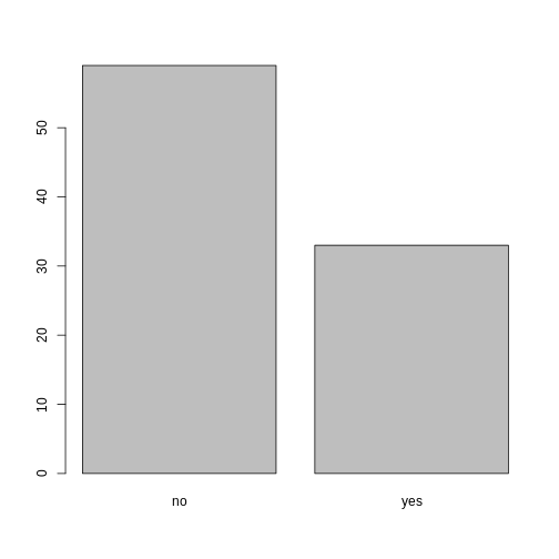
Looking at the plot compared to the output of the vector, we can see that in addition to “no”s and “yes”s, there are some respondents for whom the information about whether they were part of an irrigation association hasn’t been recorded, and encoded as missing data. These respondents do not appear on the plot. Let’s encode them differently so they can be counted and visualized in our plot.

R

## Let's recreate the vector from the data frame column "memb_assoc"
memb_assoc <- interviews$memb_assoc

## replace the missing data with "undetermined"
memb_assoc[is.na(memb_assoc)] <- "undetermined"

## convert it into a factor
memb_assoc <- as.factor(memb_assoc)

## let's see what it looks like
memb_assoc

OUTPUT

  [1] undetermined yes          undetermined undetermined undetermined
  [6] undetermined no           yes          no           no
 [11] undetermined yes          no           undetermined yes
 [16] undetermined undetermined undetermined undetermined undetermined
 [21] no           undetermined undetermined no           no
 [26] no           undetermined no           yes          undetermined
 [31] undetermined yes          no           yes          yes
 [36] yes          undetermined yes          undetermined yes
 [41] undetermined no           no           undetermined no
 [46] no           yes          undetermined undetermined yes
 [51] undetermined no           yes          no           undetermined
 [56] yes          no           no           undetermined no
 [61] yes          undetermined undetermined undetermined no
 [66] yes          no           no           no           no
 [71] yes          undetermined no           yes          undetermined
 [76] undetermined yes          no           no           yes
 [81] no           no           yes          no           yes
 [86] no           no           undetermined yes          yes
 [91] yes          yes          yes          no           no
 [96] no           no           yes          no           no
[101] yes          yes          no           undetermined no
[106] no           undetermined no           no           undetermined
[111] no           undetermined undetermined no           no
[116] no           no           yes          no           no
[121] no           no           no           no           no
[126] no           no           no           no           yes
[131] undetermined
Levels: no undetermined yes

R

summary(memb_assoc)

OUTPUT

          no undetermined          yes
          59           39           33 

R

## bar plot of the number of interview respondents who were
## members of irrigation association:
plot(memb_assoc)

Challenge

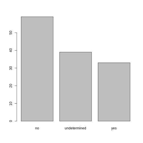
Exercise

• Rename the levels of the factor to have the first letter in uppercase: “No”,“Undetermined”, and “Yes”.

• Now that we have renamed the factor level to “Undetermined”, can you recreate the barplot such that “Undetermined” is last (after “Yes”)?

Show me the solution

R

## Rename levels.
memb_assoc <- fct_recode(memb_assoc, No = "no",
                         Undetermined = "undetermined", Yes = "yes")
## Reorder levels. Note we need to use the new level names.
memb_assoc <- factor(memb_assoc, levels = c("No", "Yes", "Undetermined"))
plot(memb_assoc)

Key Points

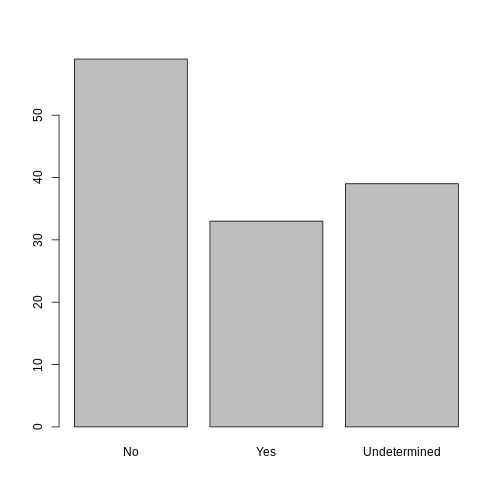
• Use read_csv to read tabular data in R.
• Use factors to represent categorical data in R.

Content from Data Wrangling with dplyr

---

Last updated on 2026-02-24 | Edit this page

Overview

Questions

• How can I select specific rows and/or columns from a dataframe?
• How can I combine multiple commands into a single command?
• How can I create new columns or remove existing columns from a dataframe?

Objectives

• Describe the purpose of an R package and the dplyr package.
• Select certain columns in a dataframe with the dplyr function select.
• Select certain rows in a dataframe according to filtering conditions with the dplyr function filter.
• Link the output of one dplyr function to the input of another function with the ‘pipe’ operator %>%.
• Add new columns to a dataframe that are functions of existing columns with mutate.
• Use the split-apply-combine concept for data analysis.
• Use summarize, group_by, and count to split a dataframe into groups of observations, apply a summary statistics for each group, and then combine the results.

• dplyr is a package for making tabular data wrangling easier by using a limited set of functions that can be combined to extract and summarize insights from your data.

• Like readr, dplyr is a part of the tidyverse. These packages were loaded in R’s memory when we called library(tidyverse) earlier.

• The package dplyr provides easy tools for the most common data wrangling tasks. It is built to work directly with dataframes, with many common tasks optimized by being written in a compiled language (C++) (not all R packages are written in R!).

There are alternatives to the tidyverse packages for data wrangling, including the package data.table. However, the tidyverse is widely used in the R community and has a consistent syntax across its packages, making it a good choice for beginners.

Learning dplyr

---

To make sure everyone will use the same dataset for this lesson, we’ll read again the SAFI dataset that we downloaded earlier.

R

## load the tidyverse
library(tidyverse)
library(here)

interviews <- read_csv(here("data", "SAFI_clean.csv"), na = "NULL")

## inspect the data
interviews

## preview the data
# view(interviews)

We’re going to learn some of the most common dplyr functions:

• select(): subset columns
• filter(): subset rows on conditions
• mutate(): create new columns by using information from other columns
• group_by() and summarize(): create summary statistics on grouped data
• arrange(): sort results
• count(): count discrete values

Selecting columns and filtering rows

---

To select columns of a dataframe, use select(). The first argument to this function is the dataframe (interviews), and the subsequent arguments are the columns to keep, separated by commas. Alternatively, if you are selecting columns adjacent to each other, you can use a : to select a range of columns, read as “select columns from ___ to ___.” You may have done something similar in the past using subsetting. select() is essentially doing the same thing as subsetting, using a package (dplyr) instead of R’s base functions.

R

# to select columns throughout the dataframe
select(interviews, village, no_membrs, months_lack_food)
# to do the same thing with subsetting
interviews[c("village","no_membrs","months_lack_food")]
# to select a series of connected columns
select(interviews, village:respondent_wall_type)

To choose rows based on specific criteria, we can use the filter() function. The argument after the dataframe is the condition we want our final dataframe to adhere to (e.g. village name is Chirodzo):

R

# filters observations where village name is "Chirodzo"
filter(interviews, village == "Chirodzo")

OUTPUT

# A tibble: 39 × 14
   key_ID village  interview_date      no_membrs years_liv respondent_wall_type
    <dbl> <chr>    <dttm>                  <dbl>     <dbl> <chr>
 1      8 Chirodzo 2016-11-16 00:00:00        12        70 burntbricks
 2      9 Chirodzo 2016-11-16 00:00:00         8         6 burntbricks
 3     10 Chirodzo 2016-12-16 00:00:00        12        23 burntbricks
 4     34 Chirodzo 2016-11-17 00:00:00         8        18 burntbricks
 5     35 Chirodzo 2016-11-17 00:00:00         5        45 muddaub
 6     36 Chirodzo 2016-11-17 00:00:00         6        23 sunbricks
 7     37 Chirodzo 2016-11-17 00:00:00         3         8 burntbricks
 8     43 Chirodzo 2016-11-17 00:00:00         7        29 muddaub
 9     44 Chirodzo 2016-11-17 00:00:00         2         6 muddaub
10     45 Chirodzo 2016-11-17 00:00:00         9         7 muddaub
# ℹ 29 more rows
# ℹ 8 more variables: rooms <dbl>, memb_assoc <chr>, affect_conflicts <chr>,
#   liv_count <dbl>, items_owned <chr>, no_meals <dbl>, months_lack_food <chr>,
#   instanceID <chr>

We can also specify multiple conditions within the filter() function. We can combine conditions using either “and” or “or” statements. In an “and” statement, an observation (row) must meet every criteria to be included in the resulting dataframe. To form “and” statements within dplyr, we can pass our desired conditions as arguments in the filter() function, separated by commas:

R

# filters observations with "and" operator (comma)
# output dataframe satisfies ALL specified conditions
filter(interviews, village == "Chirodzo",
                   rooms > 1,
                   no_meals > 2)

OUTPUT

# A tibble: 10 × 14
   key_ID village  interview_date      no_membrs years_liv respondent_wall_type
    <dbl> <chr>    <dttm>                  <dbl>     <dbl> <chr>
 1     10 Chirodzo 2016-12-16 00:00:00        12        23 burntbricks
 2     49 Chirodzo 2016-11-16 00:00:00         6        26 burntbricks
 3     52 Chirodzo 2016-11-16 00:00:00        11        15 burntbricks
 4     56 Chirodzo 2016-11-16 00:00:00        12        23 burntbricks
 5     65 Chirodzo 2016-11-16 00:00:00         8        20 burntbricks
 6     66 Chirodzo 2016-11-16 00:00:00        10        37 burntbricks
 7     67 Chirodzo 2016-11-16 00:00:00         5        31 burntbricks
 8     68 Chirodzo 2016-11-16 00:00:00         8        52 burntbricks
 9    199 Chirodzo 2017-06-04 00:00:00         7        17 burntbricks
10    200 Chirodzo 2017-06-04 00:00:00         8        20 burntbricks
# ℹ 8 more variables: rooms <dbl>, memb_assoc <chr>, affect_conflicts <chr>,
#   liv_count <dbl>, items_owned <chr>, no_meals <dbl>, months_lack_food <chr>,
#   instanceID <chr>

We can also form “and” statements with the & operator instead of commas:

R

# filters observations with "&" logical operator
# output dataframe satisfies ALL specified conditions
filter(interviews, village == "Chirodzo" &
                   rooms > 1 &
                   no_meals > 2)

OUTPUT

# A tibble: 10 × 14
   key_ID village  interview_date      no_membrs years_liv respondent_wall_type
    <dbl> <chr>    <dttm>                  <dbl>     <dbl> <chr>
 1     10 Chirodzo 2016-12-16 00:00:00        12        23 burntbricks
 2     49 Chirodzo 2016-11-16 00:00:00         6        26 burntbricks
 3     52 Chirodzo 2016-11-16 00:00:00        11        15 burntbricks
 4     56 Chirodzo 2016-11-16 00:00:00        12        23 burntbricks
 5     65 Chirodzo 2016-11-16 00:00:00         8        20 burntbricks
 6     66 Chirodzo 2016-11-16 00:00:00        10        37 burntbricks
 7     67 Chirodzo 2016-11-16 00:00:00         5        31 burntbricks
 8     68 Chirodzo 2016-11-16 00:00:00         8        52 burntbricks
 9    199 Chirodzo 2017-06-04 00:00:00         7        17 burntbricks
10    200 Chirodzo 2017-06-04 00:00:00         8        20 burntbricks
# ℹ 8 more variables: rooms <dbl>, memb_assoc <chr>, affect_conflicts <chr>,
#   liv_count <dbl>, items_owned <chr>, no_meals <dbl>, months_lack_food <chr>,
#   instanceID <chr>

In an “or” statement, observations must meet at least one of the specified conditions. To form “or” statements we use the logical operator for “or,” which is the vertical bar (|):

R

# filters observations with "|" logical operator
# output dataframe satisfies AT LEAST ONE of the specified conditions
filter(interviews, village == "Chirodzo" | village == "Ruaca")

OUTPUT

# A tibble: 88 × 14
   key_ID village  interview_date      no_membrs years_liv respondent_wall_type
    <dbl> <chr>    <dttm>                  <dbl>     <dbl> <chr>
 1      8 Chirodzo 2016-11-16 00:00:00        12        70 burntbricks
 2      9 Chirodzo 2016-11-16 00:00:00         8         6 burntbricks
 3     10 Chirodzo 2016-12-16 00:00:00        12        23 burntbricks
 4     23 Ruaca    2016-11-21 00:00:00        10        20 burntbricks
 5     24 Ruaca    2016-11-21 00:00:00         6         4 burntbricks
 6     25 Ruaca    2016-11-21 00:00:00        11         6 burntbricks
 7     26 Ruaca    2016-11-21 00:00:00         3        20 burntbricks
 8     27 Ruaca    2016-11-21 00:00:00         7        36 burntbricks
 9     28 Ruaca    2016-11-21 00:00:00         2         2 muddaub
10     29 Ruaca    2016-11-21 00:00:00         7        10 burntbricks
# ℹ 78 more rows
# ℹ 8 more variables: rooms <dbl>, memb_assoc <chr>, affect_conflicts <chr>,
#   liv_count <dbl>, items_owned <chr>, no_meals <dbl>, months_lack_food <chr>,
#   instanceID <chr>

Pipes

---

What if you want to select and filter at the same time? There are three ways to do this: use intermediate steps, nested functions, or pipes.

With intermediate steps, you create a temporary dataframe and use that as input to the next function, like this:

R

interviews2 <- filter(interviews, village == "Chirodzo")
interviews_ch <- select(interviews2, village:respondent_wall_type)

This is readable, but can clutter up your workspace with lots of objects that you have to name individually. With multiple steps, that can be hard to keep track of.

You can also nest functions (i.e. one function inside of another), like this:

R

interviews_ch <- select(filter(interviews, village == "Chirodzo"),
                         village:respondent_wall_type)

This is handy, but can be difficult to read if too many functions are nested, as R evaluates the expression from the inside out (in this case, filtering, then selecting).

The last option, pipes, are a recent addition to R. Pipes let you take the output of one function and send it directly to the next, which is useful when you need to do many things to the same dataset. You can type the pipe with:

• Ctrl + Shift + M if you have a PC or Cmd + Shift + M if you have a Mac.

R

# the following example is run using magrittr pipe but the output will be same with the native pipe
interviews %>%
    filter(village == "Chirodzo") %>%
    select(village:respondent_wall_type)

OUTPUT

# A tibble: 39 × 5
   village  interview_date      no_membrs years_liv respondent_wall_type
   <chr>    <dttm>                  <dbl>     <dbl> <chr>
 1 Chirodzo 2016-11-16 00:00:00        12        70 burntbricks
 2 Chirodzo 2016-11-16 00:00:00         8         6 burntbricks
 3 Chirodzo 2016-12-16 00:00:00        12        23 burntbricks
 4 Chirodzo 2016-11-17 00:00:00         8        18 burntbricks
 5 Chirodzo 2016-11-17 00:00:00         5        45 muddaub
 6 Chirodzo 2016-11-17 00:00:00         6        23 sunbricks
 7 Chirodzo 2016-11-17 00:00:00         3         8 burntbricks
 8 Chirodzo 2016-11-17 00:00:00         7        29 muddaub
 9 Chirodzo 2016-11-17 00:00:00         2         6 muddaub
10 Chirodzo 2016-11-17 00:00:00         9         7 muddaub
# ℹ 29 more rows

R

#interviews |>
#   filter(village == "Chirodzo") |>
#   select(village:respondent_wall_type)

In the above code, we use the pipe to send the interviews dataset first through filter() to keep rows where village is “Chirodzo”, then through select() to keep only the columns from village to respondent_wall_type. Since %>% takes the object on its left and passes it as the first argument to the function on its right, we don’t need to explicitly include the dataframe as an argument to the filter() and select() functions any more.

Some may find it helpful to read the pipe like the word “then”. For instance, in the above example, we take the dataframe interviews, then we filter for rows with village == "Chirodzo", then we select columns village:respondent_wall_type. The dplyr functions by themselves are somewhat simple, but by combining them into linear workflows with the pipe, we can accomplish more complex data wrangling operations.

If we want to create a new object with this smaller version of the data, we can assign it a new name:

R

interviews_ch <- interviews %>%
    filter(village == "Chirodzo") %>%
    select(village:respondent_wall_type)

interviews_ch

OUTPUT

# A tibble: 39 × 5
   village  interview_date      no_membrs years_liv respondent_wall_type
   <chr>    <dttm>                  <dbl>     <dbl> <chr>
 1 Chirodzo 2016-11-16 00:00:00        12        70 burntbricks
 2 Chirodzo 2016-11-16 00:00:00         8         6 burntbricks
 3 Chirodzo 2016-12-16 00:00:00        12        23 burntbricks
 4 Chirodzo 2016-11-17 00:00:00         8        18 burntbricks
 5 Chirodzo 2016-11-17 00:00:00         5        45 muddaub
 6 Chirodzo 2016-11-17 00:00:00         6        23 sunbricks
 7 Chirodzo 2016-11-17 00:00:00         3         8 burntbricks
 8 Chirodzo 2016-11-17 00:00:00         7        29 muddaub
 9 Chirodzo 2016-11-17 00:00:00         2         6 muddaub
10 Chirodzo 2016-11-17 00:00:00         9         7 muddaub
# ℹ 29 more rows

Note that the final dataframe (interviews_ch) is the leftmost part of this expression.

Challenge

Exercise

Using pipes, subset the interviews data to include interviews where respondents were members of an irrigation association (memb_assoc) and retain only the columns affect_conflicts, liv_count, and no_meals.

Show me the solution

R

interviews %>%
    filter(memb_assoc == "yes") %>%
    select(affect_conflicts, liv_count, no_meals)

OUTPUT

# A tibble: 33 × 3
   affect_conflicts liv_count no_meals
   <chr>                <dbl>    <dbl>
 1 once                     3        2
 2 never                    2        2
 3 never                    2        3
 4 once                     3        2
 5 frequently               1        3
 6 more_once                5        2
 7 more_once                3        2
 8 more_once                2        3
 9 once                     3        3
10 never                    3        3
# ℹ 23 more rows

Mutate

---

Frequently you’ll want to create new columns based on the values in existing columns, for example to do unit conversions, or to find the ratio of values in two columns. For this we’ll use mutate().

We might be interested in the ratio of number of household members to rooms used for sleeping (i.e. avg number of people per room):

R

interviews %>%
    mutate(people_per_room = no_membrs / rooms)

OUTPUT

# A tibble: 131 × 15
   key_ID village  interview_date      no_membrs years_liv respondent_wall_type
    <dbl> <chr>    <dttm>                  <dbl>     <dbl> <chr>
 1      1 God      2016-11-17 00:00:00         3         4 muddaub
 2      2 God      2016-11-17 00:00:00         7         9 muddaub
 3      3 God      2016-11-17 00:00:00        10        15 burntbricks
 4      4 God      2016-11-17 00:00:00         7         6 burntbricks
 5      5 God      2016-11-17 00:00:00         7        40 burntbricks
 6      6 God      2016-11-17 00:00:00         3         3 muddaub
 7      7 God      2016-11-17 00:00:00         6        38 muddaub
 8      8 Chirodzo 2016-11-16 00:00:00        12        70 burntbricks
 9      9 Chirodzo 2016-11-16 00:00:00         8         6 burntbricks
10     10 Chirodzo 2016-12-16 00:00:00        12        23 burntbricks
# ℹ 121 more rows
# ℹ 9 more variables: rooms <dbl>, memb_assoc <chr>, affect_conflicts <chr>,
#   liv_count <dbl>, items_owned <chr>, no_meals <dbl>, months_lack_food <chr>,
#   instanceID <chr>, people_per_room <dbl>

Challenge

Exercise

Create a new dataframe from the interviews data that meets the following criteria: contains only the village column and a new column called total_meals containing a value that is equal to the total number of meals served in the household per day on average (no_membrs times no_meals). Only the rows where total_meals is greater than 20 should be shown in the final dataframe.

Hint: think about how the commands should be ordered to produce this data frame!

Show me the solution

R

interviews_total_meals <- interviews %>%
    mutate(total_meals = no_membrs * no_meals) %>%
    filter(total_meals > 20) %>%
    select(village, total_meals)

Split-apply-combine data analysis and the summarize() function

---

Many data analysis tasks can be approached using the split-apply-combine paradigm: split the data into groups, apply some analysis to each group, and then combine the results. dplyr makes this very easy through the use of the group_by() function.

The summarize() function

group_by() is often used together with summarize(), which collapses each group into a single-row summary of that group. group_by() takes as arguments the column names that contain the categorical variables for which you want to calculate the summary statistics. So to compute the average household size by village:

R

interviews %>%
    group_by(village) %>%
    summarize(mean_no_membrs = mean(no_membrs))

OUTPUT

# A tibble: 3 × 2
  village  mean_no_membrs
  <chr>             <dbl>
1 Chirodzo           7.08
2 God                6.86
3 Ruaca              7.57

You can also group by multiple columns: In that case we will get the average household size for each combination of village and membership in an irrigation association:

R

interviews %>%
    group_by(village, memb_assoc) %>%
    summarize(mean_no_membrs = mean(no_membrs))

OUTPUT

`summarise()` has grouped output by 'village'. You can override using the
`.groups` argument.

OUTPUT

# A tibble: 9 × 3
# Groups:   village [3]
  village  memb_assoc mean_no_membrs
  <chr>    <chr>               <dbl>
1 Chirodzo no                   8.06
2 Chirodzo yes                  7.82
3 Chirodzo <NA>                 5.08
4 God      no                   7.13
5 God      yes                  8
6 God      <NA>                 6
7 Ruaca    no                   7.18
8 Ruaca    yes                  9.5
9 Ruaca    <NA>                 6.22

Note that the output is a grouped tibble of nine rows by three columns which is indicated by the by two first lines with the #. To obtain an ungrouped tibble, use the ungroup function:

R

interviews %>%
    group_by(village, memb_assoc) %>%
    summarize(mean_no_membrs = mean(no_membrs)) %>%
    ungroup()

OUTPUT

`summarise()` has grouped output by 'village'. You can override using the
`.groups` argument.

OUTPUT

# A tibble: 9 × 3
  village  memb_assoc mean_no_membrs
  <chr>    <chr>               <dbl>
1 Chirodzo no                   8.06
2 Chirodzo yes                  7.82
3 Chirodzo <NA>                 5.08
4 God      no                   7.13
5 God      yes                  8
6 God      <NA>                 6
7 Ruaca    no                   7.18
8 Ruaca    yes                  9.5
9 Ruaca    <NA>                 6.22

Notice that the second line with the # that previously indicated the grouping has disappeared and we now only have a 9x3-tibble without grouping. When grouping both by village and membr_assoc, we see rows in our table for respondents who did not specify whether they were a member of an irrigation association. We can exclude those data from our table using a filter step.

R

interviews %>%
    filter(!is.na(memb_assoc)) %>%
    group_by(village, memb_assoc) %>%
    summarize(mean_no_membrs = mean(no_membrs))

OUTPUT

`summarise()` has grouped output by 'village'. You can override using the
`.groups` argument.

OUTPUT

# A tibble: 6 × 3
# Groups:   village [3]
  village  memb_assoc mean_no_membrs
  <chr>    <chr>               <dbl>
1 Chirodzo no                   8.06
2 Chirodzo yes                  7.82
3 God      no                   7.13
4 God      yes                  8
5 Ruaca    no                   7.18
6 Ruaca    yes                  9.5 

Once the data are grouped, you can also summarize multiple variables at the same time (and not necessarily on the same variable). For instance, we could add a column indicating the minimum household size for each village for each group (members of an irrigation association vs not):

R

interviews %>%
    filter(!is.na(memb_assoc)) %>%
    group_by(village, memb_assoc) %>%
    summarize(mean_no_membrs = mean(no_membrs),
              min_membrs = min(no_membrs))

OUTPUT

`summarise()` has grouped output by 'village'. You can override using the
`.groups` argument.

OUTPUT

# A tibble: 6 × 4
# Groups:   village [3]
  village  memb_assoc mean_no_membrs min_membrs
  <chr>    <chr>               <dbl>      <dbl>
1 Chirodzo no                   8.06          4
2 Chirodzo yes                  7.82          2
3 God      no                   7.13          3
4 God      yes                  8             5
5 Ruaca    no                   7.18          2
6 Ruaca    yes                  9.5           5

It is sometimes useful to rearrange the result of a query to inspect the values. For instance, we can sort on min_membrs to put the group with the smallest household first:

R

interviews %>%
    filter(!is.na(memb_assoc)) %>%
    group_by(village, memb_assoc) %>%
    summarize(mean_no_membrs = mean(no_membrs),
              min_membrs = min(no_membrs)) %>%
    arrange(min_membrs)

OUTPUT

`summarise()` has grouped output by 'village'. You can override using the
`.groups` argument.

OUTPUT

# A tibble: 6 × 4
# Groups:   village [3]
  village  memb_assoc mean_no_membrs min_membrs
  <chr>    <chr>               <dbl>      <dbl>
1 Chirodzo yes                  7.82          2
2 Ruaca    no                   7.18          2
3 God      no                   7.13          3
4 Chirodzo no                   8.06          4
5 God      yes                  8             5
6 Ruaca    yes                  9.5           5

To sort in descending order, we need to add the desc() function. If we want to sort the results by decreasing order of minimum household size:

R

interviews %>%
    filter(!is.na(memb_assoc)) %>%
    group_by(village, memb_assoc) %>%
    summarize(mean_no_membrs = mean(no_membrs),
              min_membrs = min(no_membrs)) %>%
    arrange(desc(min_membrs))

OUTPUT

`summarise()` has grouped output by 'village'. You can override using the
`.groups` argument.

OUTPUT

# A tibble: 6 × 4
# Groups:   village [3]
  village  memb_assoc mean_no_membrs min_membrs
  <chr>    <chr>               <dbl>      <dbl>
1 God      yes                  8             5
2 Ruaca    yes                  9.5           5
3 Chirodzo no                   8.06          4
4 God      no                   7.13          3
5 Chirodzo yes                  7.82          2
6 Ruaca    no                   7.18          2

Counting

When working with data, we often want to know the number of observations found for each factor or combination of factors. For this task, dplyr provides count(). For example, if we wanted to count the number of rows of data for each village, we would do:

R

interviews %>%
    count(village)

OUTPUT

# A tibble: 3 × 2
  village      n
  <chr>    <int>
1 Chirodzo    39
2 God         43
3 Ruaca       49

For convenience, count() provides the sort argument to get results in decreasing order:

R

interviews %>%
    count(village, sort = TRUE)

OUTPUT

# A tibble: 3 × 2
  village      n
  <chr>    <int>
1 Ruaca       49
2 God         43
3 Chirodzo    39

Challenge

Exercise

How many households in the survey have an average of two meals per day? Three meals per day? Are there any other numbers of meals represented?

Show me the solution

R

interviews %>%
   count(no_meals)

OUTPUT

# A tibble: 2 × 2
  no_meals     n
     <dbl> <int>
1        2    52
2        3    79

Challenge

Exercise (continued)

Use group_by() and summarize() to find the mean, min, and max number of household members for each village. Also add the number of observations (hint: see ?n).

Show me the solution

R

interviews %>%
  group_by(village) %>%
  summarize(
      mean_no_membrs = mean(no_membrs),
      min_no_membrs = min(no_membrs),
      max_no_membrs = max(no_membrs),
      n = n()
  )

OUTPUT

# A tibble: 3 × 5
  village  mean_no_membrs min_no_membrs max_no_membrs     n
  <chr>             <dbl>         <dbl>         <dbl> <int>
1 Chirodzo           7.08             2            12    39
2 God                6.86             3            15    43
3 Ruaca              7.57             2            19    49

Challenge

Exercise (continued)

What was the largest household interviewed in each month?

Show me the solution

R

# if not already included, add month, year, and day columns
library(lubridate) # load lubridate if not already loaded
interviews %>%
    mutate(month = month(interview_date),
           day = day(interview_date),
           year = year(interview_date)) %>%
    group_by(year, month) %>%
    summarize(max_no_membrs = max(no_membrs))

OUTPUT

`summarise()` has grouped output by 'year'. You can override using the
`.groups` argument.

OUTPUT

# A tibble: 5 × 3
# Groups:   year [2]
   year month max_no_membrs
  <dbl> <dbl>         <dbl>
1  2016    11            19
2  2016    12            12
3  2017     4            17
4  2017     5            15
5  2017     6            15

Key Points

• Use the dplyr package to manipulate dataframes.
• Use select() to choose variables from a dataframe.
• Use filter() to choose data based on values.
• Use group_by() and summarize() to work with subsets of data.
• Use mutate() to create new variables.

Content from Data Visualisation with ggplot2

---

Last updated on 2026-02-24 | Edit this page

Overview

Questions

• What are the components of a ggplot?
• What are the main differences between R base plots, lattice, and ggplot?
• How do I create scatterplots, boxplots, and barplots?
• How can I change the aesthetics (ex. colour, transparency) of my plot?
• How can I create multiple plots at once?

Objectives

• Produce scatter plots, boxplots, and barplots using ggplot.
• Set universal plot settings.
• Describe what faceting is and apply faceting in ggplot.
• Modify the aesthetics of an existing ggplot plot (including axis labels and colour).
• Build complex and customized plots from data in a data frame.
• Recognize the differences between base R, lattice, and ggplot visualizations.

We start by loading the required package. ggplot2 is also included in the tidyverse package.

R

library(tidyverse)
# library(ggplot2) # If you don't want to load the whole tidyverse, you can just load ggplot2

If not still in the workspace, load the data we just downloaded/saved in the previous lesson.

R

interviews_plotting <- read_csv("data_output/interviews_plotting.csv")

OUTPUT

Rows: 131 Columns: 45
── Column specification ────────────────────────────────────────────────────────
Delimiter: ","
chr   (5): village, respondent_wall_type, memb_assoc, affect_conflicts, inst...
dbl   (8): key_ID, no_membrs, years_liv, rooms, liv_count, no_meals, number_...
lgl  (31): bicycle, television, solar_panel, table, cow_cart, radio, cow_plo...
dttm  (1): interview_date

ℹ Use `spec()` to retrieve the full column specification for this data.
ℹ Specify the column types or set `show_col_types = FALSE` to quiet this message.

If you were unable to complete the previous lesson or did not save the data, then you can create it now. Either download it using read_csv() (Option 1) or create it with the dplyr and tidyr code (Option 2).

Option 1: Download the data

Option 2: Create the data

R

interviews_plotting <- read_csv("https://raw.githubusercontent.com/datacarpentry/r-socialsci/main/episodes/data/interviews_plotting.csv")

R

## Can be used to load in data from previous lesson!
interviews_plotting <- interviews %>%
  ## pivot wider by items_owned
  separate_longer_delim(items_owned, delim = ";") %>%
  replace_na(list(items_owned = "no_listed_items")) %>%
  ## Use of grouped mutate to find number of rows
  group_by(key_ID) %>% 
  mutate(items_owned_logical = TRUE,
         number_items = if_else(items_owned == "no_listed_items", 0, n())) %>% 
  pivot_wider(names_from = items_owned,
              values_from = items_owned_logical,
              values_fill = list(items_owned_logical = FALSE)) %>% 
  ## pivot wider by months_lack_food
  separate_longer_delim(months_lack_food, delim = ";") %>%
  mutate(months_lack_food_logical = TRUE,
         number_months_lack_food = if_else(months_lack_food == "none", 0, n())) %>%
  pivot_wider(names_from = months_lack_food,
              values_from = months_lack_food_logical,
              values_fill = list(months_lack_food_logical = FALSE))

This code takes the original interviews dataset and transforms it to make it easier to analyze and visualize with ggplot2. The result is a dataset where each respondent has columns for each possible item and month, making it much easier to summarize, count, and plot ownership or food insecurity patterns across the sample

Visualization Options in R

---

Before we start with ggplot2, it’s helpful to know that there are several ways to create visualizations in R. While ggplot2 is great for building complex and highly customizable plots, there are simpler and quicker alternatives that you might encounter or use depending on the context. Let’s briefly explore a few of them:

R Base Plots

Base R plots are the simplest form of visualization and are great for quick, exploratory analysis. You can create plots with very little code, but customizing them can be cumbersome compared to ggplot2.

Example of a simple scatterplot in base R using the no_membrs and liv_count variables:

R

plot(interviews_plotting$no_membrs, interviews_plotting$liv_count,
     main = "Base R Scatterplot",
     xlab = "Number of Household Members",
     ylab = "Number of Livestock Owned")

Lattice (optional)

Lattice is another plotting system in R, which allows for creating multi-panel plots easily. It’s different from ggplot2 because you define the entire plot in a single function call, and modifications after plotting are limited.

Example of a lattice plot using no_membrs and liv_count split by village:

R

library(lattice)

R

xyplot(liv_count ~ no_membrs | village, data = interviews_plotting,
       main = "Lattice Plot: Livestock Count by Household Members",
       xlab = "Number of Household Members",
       ylab = "Number of Livestock Owned")

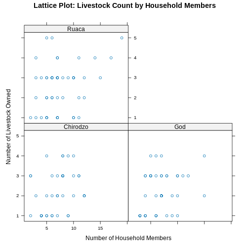
Plotting with ggplot2

---

ggplot2 is a plotting package that makes it simple to create complex plots from data stored in a data frame. It provides a programmatic interface for specifying what variables to plot, how they are displayed, and general visual properties. Therefore, we only need minimal changes if the underlying data change or if we decide to change from a bar plot to a scatterplot. This helps in creating publication quality plots with minimal amounts of adjustments and tweaking.

ggplot2 functions work best with data in the ‘long’ format, i.e., a column for every dimension, and a row for every observation. Well-structured data will save you lots of time when making figures with ggplot2

ggplot graphics are built step by step by adding new elements. Adding layers in this fashion allows for extensive flexibility and customization of plots.

Each chart built with ggplot2 must include the following

• Data

• Aesthetic mapping (aes)

  • Describes how variables are mapped onto graphical attributes
  • Visual attribute of data including x-y axes, color, fill, shape, and alpha

• Geometric objects (geom)

  • Determines how values are rendered graphically, as bars (geom_bar), scatterplot (geom_point), line (geom_line), etc.

Thus, the template for graphic in ggplot2 is:

<DATA> %>%
    ggplot(aes(<MAPPINGS>)) +
    <GEOM_FUNCTION>()

Remember from the last lesson that the pipe operator %>% places the result of the previous line(s) into the first argument of the function. ggplot is a function that expects a data frame to be the first argument. This allows for us to change from specifying the data = argument within the ggplot function and instead pipe the data into the function.

• use the ggplot() function and bind the plot to a specific data frame.

R

interviews_plotting %>%
    ggplot()

• define a mapping (using the aesthetic (aes) function), by selecting the variables to be plotted and specifying how to present them in the graph, e.g. as x/y positions or characteristics such as size, shape, color, etc.

R

interviews_plotting %>%
    ggplot(aes(x = no_membrs, y = number_items))

• add ‘geoms’ – graphical representations of the data in the plot (points, lines, bars). ggplot2 offers many different geoms; we will use some common ones today, including:

  • geom_point() for scatter plots, dot plots, etc.
  • geom_boxplot() for, well, boxplots!
  • geom_line() for trend lines, time series, etc.

To add a geom to the plot use the + operator. Because we have two continuous variables, let’s use geom_point() first:

R

interviews_plotting %>%
    ggplot(aes(x = no_membrs, y = number_items)) +
    geom_point()

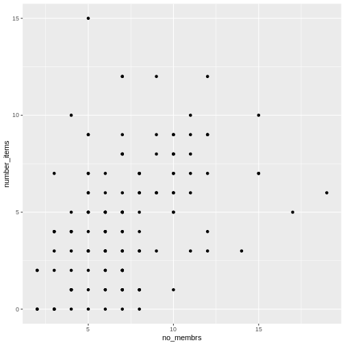
The + in the ggplot2 package is particularly useful because it allows you to modify existing ggplot objects. This means you can easily set up plot templates and conveniently explore different types of plots, so the above plot can also be generated with code like this, similar to the “intermediate steps” approach in the previous lesson:

R

# Assign plot to a variable
interviews_plot <- interviews_plotting %>%
    ggplot(aes(x = no_membrs, y = number_items))

# Draw the plot as a dot plot
interviews_plot +
    geom_point()

Callout

Notes

• Anything you put in the ggplot() function can be seen by any geom layers that you add (i.e., these are universal plot settings). This includes the x- and y-axis mapping you set up in aes().
• You can also specify mappings for a given geom independently of the mapping defined globally in the ggplot() function.
• The + sign used to add new layers must be placed at the end of the line containing the previous layer. If, instead, the + sign is added at the beginning of the line containing the new layer, ggplot2 will not add the new layer and will return an error message.

R

## This is the correct syntax for adding layers
interviews_plot +
    geom_point()

## This will not add the new layer and will return an error message
interviews_plot
+ geom_point()

Building your plots iteratively

---

Building plots with ggplot2 is typically an iterative process. We start by defining the dataset we’ll use, lay out the axes, and choose a geom:

R

interviews_plotting %>%
    ggplot(aes(x = no_membrs, y = number_items)) +
    geom_point()

Then, we start modifying this plot to extract more information from it. For instance, when inspecting the plot we notice that points only appear at the intersection of whole numbers of no_membrs and number_items. Also, from a rough estimate, it looks like there are far fewer dots on the plot than there rows in our dataframe. This should lead us to believe that there may be multiple observations plotted on top of each other (e.g. three observations where no_membrs is 3 and number_items is 1).

There are two main ways to alleviate overplotting issues:

1. changing the transparency of the points
2. jittering the location of the points

Let’s first explore option 1, changing the transparency of the points. What we mean when we say “transparency” we mean the opacity of point, or your ability to see through the point. We can control the transparency of the points with the alpha argument to geom_point. Values of alpha range from 0 to 1, with lower values corresponding to more transparent colors (an alpha of 1 is the default value). Specifically, an alpha of 0.1, would make a point one-tenth as opaque as a normal point. Stated differently ten points stacked on top of each other would correspond to a normal point.

Here, we change the alpha to 0.5, in an attempt to help fix the overplotting. While the overplotting isn’t solved, adding transparency begins to address this problem, as the points where there are overlapping observations are darker (as opposed to lighter gray):

R

interviews_plotting %>%
    ggplot(aes(x = no_membrs, y = number_items)) +
    geom_point(alpha = 0.5)

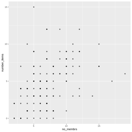
That only helped a little bit with the overplotting problem, so let’s try option two. We can jitter the points on the plot, so that we can see each point in the locations where there are overlapping points. Jittering introduces a little bit of randomness into the position of our points. You can think of this process as taking the overplotted graph and giving it a tiny shake. The points will move a little bit side-to-side and up-and-down, but their position from the original plot won’t dramatically change. Note that this solution is suitable for plotting integer figures, while for numeric figures with decimals, geom_jitter() becomes inappropriate because it obscures the true value of the observation.

We can jitter our points using the geom_jitter() function instead of the geom_point() function, as seen below:

R

interviews_plotting %>%
    ggplot(aes(x = no_membrs, y = number_items)) +
    geom_jitter()

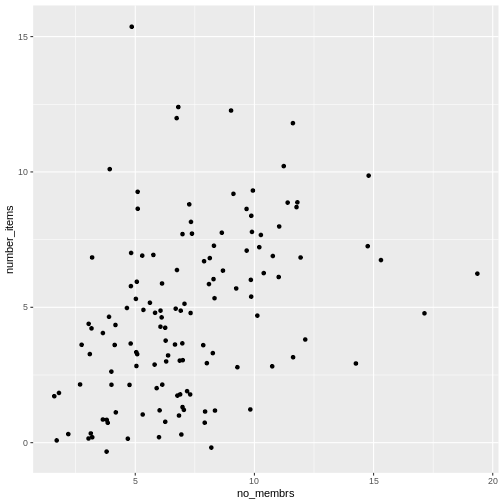
The geom_jitter() function allows for us to specify the amount of random motion in the jitter, using the width and height arguments. When we don’t specify values for width and height, geom_jitter() defaults to 40% of the resolution of the data (the smallest change that can be measured). Hence, if we would like less spread in our jitter than was default, we should pick values between 0.1 and 0.4. Experiment with the values to see how your plot changes.

R

interviews_plotting %>%
    ggplot(aes(x = no_membrs, y = number_items)) +
    geom_jitter(alpha = 0.5,
                width = 0.2,
                height = 0.2)

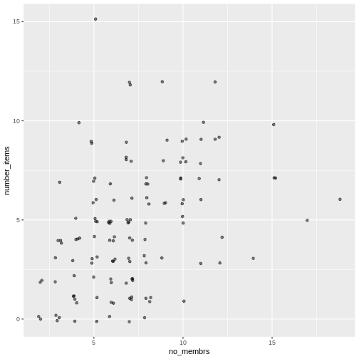
For our final change, we can also add colours for all the points by specifying a color argument inside the geom_jitter() function:

R

interviews_plotting %>%
    ggplot(aes(x = no_membrs, y = number_items)) +
    geom_jitter(alpha = 0.5,
                color = "blue",
                width = 0.2,
                height = 0.2)

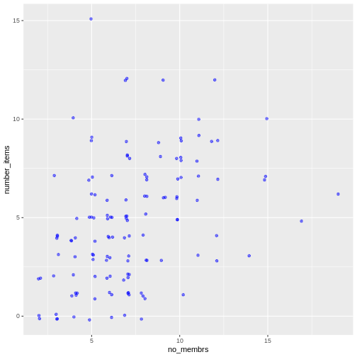
To colour each village in the plot differently, you could use a vector as an input to the argument color. However, because we are now mapping features of the data to a colour, instead of setting one colour for all points, the colour of the points now needs to be set inside a call to the aes function. When we map a variable in our data to the colour of the points, ggplot2 will provide a different colour corresponding to the different values of the variable. We will continue to specify the value of alpha, width, and height outside of the aes function because we are using the same value for every point. ggplot2 understands both the Commonwealth English and American English spellings for colour, i.e., you can use either color or colour. Here is an example where we color points by the village of the observation:

R

interviews_plotting %>%
    ggplot(aes(x = no_membrs, y = number_items)) +
    geom_jitter(aes(color = village), alpha = 0.5, width = 0.2, height = 0.2)

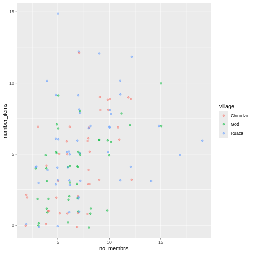
There appears to be a positive trend between number of household members and number of items owned (from the list provided). Additionally, this trend does not appear to be different by village.

Callout

Notes

As you will learn, there are multiple ways to plot the a relationship between variables. Another way to plot data with overlapping points is to use the geom_count plotting function. The geom_count() function makes the size of each point representative of the number of data items of that type and the legend gives point sizes associated to particular numbers of items.

R

interviews_plotting %>%
   ggplot(aes(x = no_membrs, y = number_items, color = village)) +
   geom_count()

Challenge

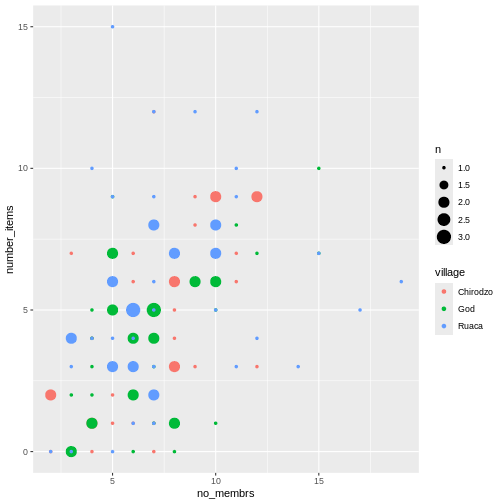
Exercise

Use what you just learned to create a scatter plot of rooms by village with the respondent_wall_type showing in different colours. Does this seem like a good way to display the relationship between these variables? What other kinds of plots might you use to show this type of data?

Show me the solution

R

interviews_plotting %>%
    ggplot(aes(x = village, y = rooms)) +
    geom_jitter(aes(color = respondent_wall_type),
      alpha = 0.5,
        width = 0.2,
        height = 0.2)

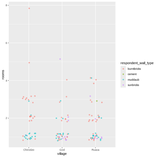
This is not a great way to show this type of data because it is difficult to distinguish between villages. What other plot types could help you visualize this relationship better?

Boxplot and violin plots

---

We can use boxplots to visualize the distribution of rooms for each wall type:

R

interviews_plotting %>%
    ggplot(aes(x = respondent_wall_type, y = rooms)) +
    geom_boxplot()

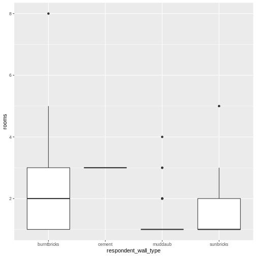
By adding points to a boxplot, we can have a better idea of the number of measurements and of their distribution:

R

interviews_plotting %>%
    ggplot(aes(x = respondent_wall_type, y = rooms)) +
    geom_boxplot(alpha = 0) +
    geom_jitter(alpha = 0.5,
        color = "tomato",
        width = 0.2,
        height = 0.2)

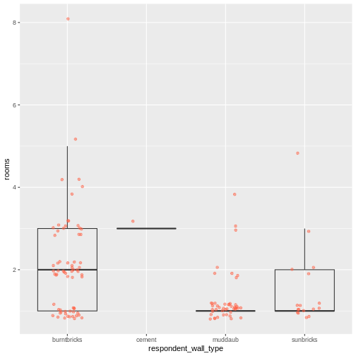
We can see that muddaub houses and sunbrick houses tend to be smaller than burntbrick houses.

Notice how the boxplot layer is behind the jitter layer? What do you need to change in the code to put the boxplot layer in front of the jitter layer?

Violin plots are another way to visualize the distribution of a variable. They are similar to boxplots, but they also show the density of the data at different values. This can be useful for understanding the shape of the distribution, especially when there are multiple modes (peaks) in the data.

Challenge

Exercise

Boxplots are useful summaries, but hide the shape of the distribution. For example, if the distribution is bimodal, we would not see it in a boxplot. An alternative to the boxplot is the violin plot, where the shape (of the density of points) is drawn.

• Replace the box plot with a violin plot; see geom_violin().

Show me the solution

R

interviews_plotting %>%
  ggplot(aes(x = respondent_wall_type, y = rooms)) +
  geom_violin(alpha = 0) +
  geom_jitter(alpha = 0.5, color = "tomato")

WARNING

Warning: Groups with fewer than two datapoints have been dropped.
ℹ Set `drop = FALSE` to consider such groups for position adjustment purposes.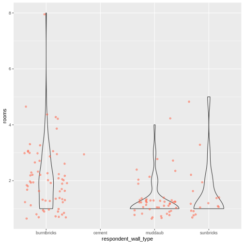

Challenge

Exercise (continued)

So far, we’ve looked at the distribution of room number within wall type. Try making a new plot to explore the distribution of another variable within wall type.

• Create a boxplot for liv_count for each wall type. Overlay the boxplot layer on a jitter layer to show actual measurements.

Show me the solution

R

interviews_plotting %>%
   ggplot(aes(x = respondent_wall_type, y = liv_count)) +
   geom_boxplot(alpha = 0) +
   geom_jitter(alpha = 0.5, width = 0.2, height = 0.2)

Challenge

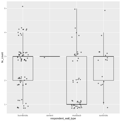
Exercise (continued)

• Add colour to the data points on your boxplot according to whether the respondent is a member of an irrigation association (memb_assoc).

Show me the solution

R

interviews_plotting %>%
  ggplot(aes(x = respondent_wall_type, y = liv_count)) +
  geom_boxplot(alpha = 0) +
  geom_jitter(aes(color = memb_assoc), alpha = 0.5, width = 0.2, height = 0.2)

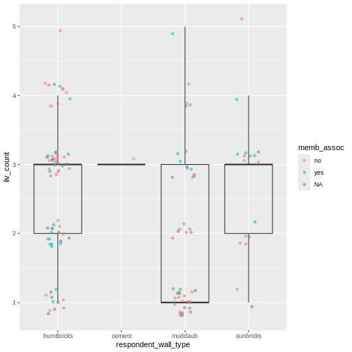
Barplots

---

Barplots are also useful for visualizing categorical data. By default, geom_bar accepts a variable for x, and plots the number of instances each value of x (in this case, wall type) appears in the dataset.

R

interviews_plotting %>%
    ggplot(aes(x = respondent_wall_type)) +
    geom_bar()

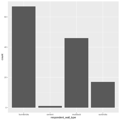
We can use the fill aesthetic for the geom_bar() geom to colour bars by the portion of each count that is from each village.

R

interviews_plotting %>%
    ggplot(aes(x = respondent_wall_type)) +
    geom_bar(aes(fill = village))

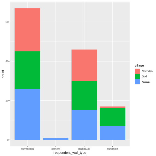
This creates a stacked bar chart. These are generally more difficult to read than side-by-side bars. We can separate the portions of the stacked bar that correspond to each village and put them side-by-side by using the position argument for geom_bar() and setting it to “dodge”.

R

interviews_plotting %>%
    ggplot(aes(x = respondent_wall_type)) +
    geom_bar(aes(fill = village), position = "dodge")

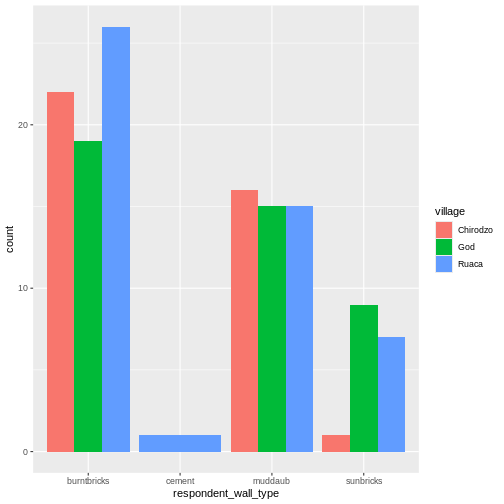
This is a nicer graphic, but we’re more likely to be interested in the proportion of each housing type in each village than in the actual count of number of houses of each type (because we might have sampled different numbers of households in each village). To compare proportions, we will first create a new data frame (percent_wall_type) with a new column named “percent” representing the percent of each house type in each village. We will remove houses with cement walls, as there was only one in the dataset.

R

percent_wall_type <- interviews_plotting %>%
    filter(respondent_wall_type != "cement") %>%
    count(village, respondent_wall_type) %>%
    group_by(village) %>%
    mutate(percent = (n / sum(n)) * 100) %>%
    ungroup()

Now we can use this new data frame to create our plot showing the percentage of each house type in each village.

R

percent_wall_type %>%
    ggplot(aes(x = village, y = percent, fill = respondent_wall_type)) +
    geom_bar(stat = "identity", position = "dodge")

Challenge

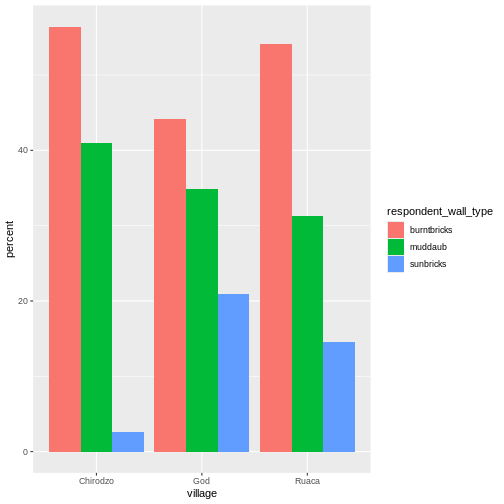
Exercise

Create a bar plot showing the proportion of respondents in each village who are or are not part of an irrigation association (memb_assoc). Include only respondents who answered that question in the calculations and plot. Which village had the lowest proportion of respondents in an irrigation association?

Show me the solution

R

percent_memb_assoc <- interviews_plotting %>%
  filter(!is.na(memb_assoc)) %>%
  count(village, memb_assoc) %>%
  group_by(village) %>%
  mutate(percent = (n / sum(n)) * 100) %>%
  ungroup()

percent_memb_assoc %>%
   ggplot(aes(x = village, y = percent, fill = memb_assoc)) +
    geom_bar(stat = "identity", position = "dodge")

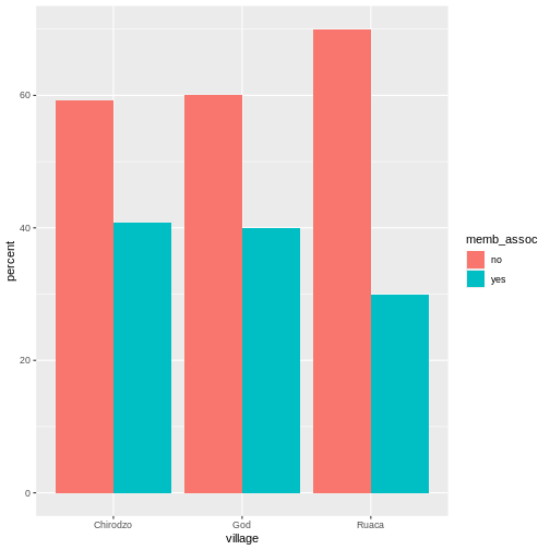
Ruaca had the lowest proportion of members in an irrigation association.

Adding Labels and Titles

---

By default, the axes labels on a plot are determined by the name of the variable being plotted. However, ggplot2 offers lots of customization options, like specifying the axes labels, and adding a title to the plot with relatively few lines of code. We will add more informative x-and y-axis labels to our plot, a more explanatory label to the legend, and a plot title.

The labs function takes the following arguments:

• title – to produce a plot title
• subtitle – to produce a plot subtitle (smaller text placed beneath the title)
• caption – a caption for the plot
• ... – any pair of name and value for aesthetics used in the plot (e.g., x, y, fill, color, size)

R

percent_wall_type %>%
    ggplot(aes(x = village, y = percent, fill = respondent_wall_type)) +
    geom_bar(stat = "identity", position = "dodge") +
    labs(title = "Proportion of wall type by village",
         fill = "Type of Wall in Home",
         x = "Village",
         y = "Percent")

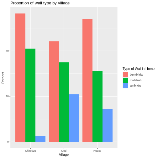
Faceting

---

Rather than creating a single plot with side-by-side bars for each village, we may want to create multiple plot, where each plot shows the data for a single village. This would be especially useful if we had a large number of villages that we had sampled, as a large number of side-by-side bars will become more difficult to read.

ggplot2 has a special technique called faceting that allows the user to split one plot into multiple plots based on a factor included in the dataset. We will use it to split our barplot of housing type proportion by village so that each village has its own panel in a multi-panel plot:

R

percent_wall_type %>%
    ggplot(aes(x = respondent_wall_type, y = percent)) +
    geom_bar(stat = "identity", position = "dodge") +
    labs(title="Proportion of wall type by village",
         x="Wall Type",
         y="Percent") +
    facet_wrap(~ village)

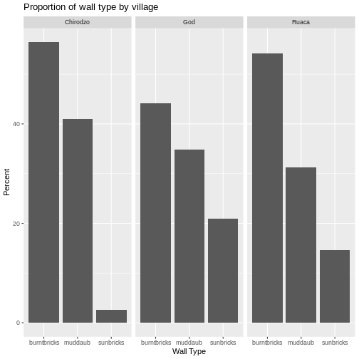
Click the “Zoom” button in your RStudio plots pane to view a larger version of this plot.

Usually plots with white background look more readable when printed. We can set the background to white using the function theme_bw(). Additionally, you can remove the grid:

R

percent_wall_type %>%
    ggplot(aes(x = respondent_wall_type, y = percent)) +
    geom_bar(stat = "identity", position = "dodge") +
    labs(title="Proportion of wall type by village",
         x="Wall Type",
         y="Percent") +
    facet_wrap(~ village) +
    theme_bw() +
    theme(panel.grid = element_blank())

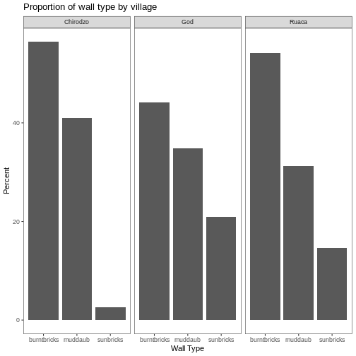
• If you want to save the plot, you can also use the ggsave() function to save your plot directly from R. For example:

R

my_plot <- percent_wall_type %>%
    ggplot(aes(x = respondent_wall_type, y = percent)) +
    geom_bar(stat = "identity", position = "dodge") +
    labs(title="Proportion of wall type by village",
         x="Wall Type",
         y="Percent") +
    facet_wrap(~ village) +
    theme_bw() +
    theme(panel.grid = element_blank())
ggsave("fig_output/name_of_file.png", my_plot, width = 15, height = 10)

ERROR

Error in `ggsave()`:
! Cannot find directory 'fig_output'.
ℹ Please supply an existing directory or use `create.dir = TRUE`.

Self paced exercise

---

What if we wanted to see the proportion of respondents in each village who owned a particular item? We can calculate the percent of people in each village who own each item and then create a faceted series of bar plots where each plot is a particular item. First we need to calculate the percentage of people in each village who own each item:

R

percent_items <- interviews_plotting %>%
    group_by(village) %>%
    summarize(across(bicycle:no_listed_items, ~ sum(.x) / n() * 100)) %>%
    pivot_longer(bicycle:no_listed_items, names_to = "items", values_to = "percent")

To calculate this percentage data frame, we needed to use the across() function within a summarize() operation. Unlike the previous example with a single wall type variable, where each response was exactly one of the types specified, people can (and do) own more than one item. So there are multiple columns of data (one for each item), and the percentage calculation needs to be repeated for each column.

Combining summarize() with across() allows us to specify first, the columns to be summarized (bicycle:no_listed_items) and then the calculation. Because our calculation is a bit more complex than is available in a built-in function, we define a new formula:

• ~ indicates that we are defining a formula,
• sum(.x) gives the number of people owning that item by counting the number of TRUE values (.x is shorthand for the column being operated on),
• and n() gives the current group size.

After the summarize() operation, we have a table of percentages with each item in its own column, so a pivot_longer() is required to transform the table into an easier format for plotting. Using this data frame, we can now create a multi-paneled bar plot.

R

percent_items %>%
    ggplot(aes(x = village, y = percent)) +
    geom_bar(stat = "identity", position = "dodge") +
    facet_wrap(~ items) +
    theme_bw() +
    theme(panel.grid = element_blank())

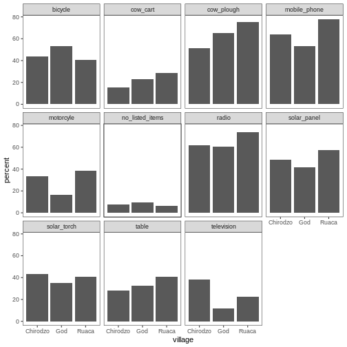
ggplot2 themes

---

In addition to theme_bw(), which changes the plot background to white, ggplot2 comes with several other themes which can be useful to quickly change the look of your visualization. The complete list of themes is available at https://ggplot2.tidyverse.org/reference/ggtheme.html. theme_minimal() and theme_light() are popular, and theme_void() can be useful as a starting point to create a new hand-crafted theme.

The ggthemes package provides a wide variety of options (including an Excel 2003 theme). The ggplot2 extensions website provides a list of packages that extend the capabilities of ggplot2, including additional themes.

Discussion

Exercise

Experiment with at least two different themes. Build the previous plot using each of those themes. Which do you like best?

Customization

---

Take a look at the ggplot2 cheat sheet, and think of ways you could improve the plot.

Now, let’s change names of axes to something more informative than ‘village’ and ‘percent’ and add a title to the figure:

R

percent_items %>%
    ggplot(aes(x = village, y = percent)) +
    geom_bar(stat = "identity", position = "dodge") +
    facet_wrap(~ items) +
    labs(title = "Percent of respondents in each village who owned each item",
         x = "Village",
         y = "Percent of Respondents") +
    theme_bw()

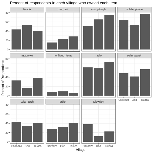
The axes have more informative names, but their readability can be improved by increasing the font size:

R

percent_items %>%
    ggplot(aes(x = village, y = percent)) +
    geom_bar(stat = "identity", position = "dodge") +
    facet_wrap(~ items) +
    labs(title = "Percent of respondents in each village who owned each item",
         x = "Village",
         y = "Percent of Respondents") +
    theme_bw() +
    theme(text = element_text(size = 16))

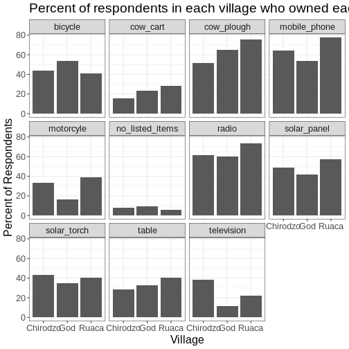
Note that it is also possible to change the fonts of your plots. If you are on Windows, you may have to install the extrafont package, and follow the instructions included in the README for this package.

After our manipulations, you may notice that the values on the x-axis are still not properly readable. Let’s change the orientation of the labels and adjust them vertically and horizontally so they don’t overlap. You can use a 90-degree angle, or experiment to find the appropriate angle for diagonally oriented labels. With a larger font, the title also runs off. We can add “\n” in the string for the title to insert a new line:

R

percent_items %>%
    ggplot(aes(x = village, y = percent)) +
    geom_bar(stat = "identity", position = "dodge") +
    facet_wrap(~ items) +
    labs(title = "Percent of respondents in each village \n who owned each item",
         x = "Village",
         y = "Percent of Respondents") +
    theme_bw() +
    theme(axis.text.x = element_text(colour = "grey20", size = 12, angle = 45,
                                     hjust = 0.5, vjust = 0.5),
          axis.text.y = element_text(colour = "grey20", size = 12),
          text = element_text(size = 16))

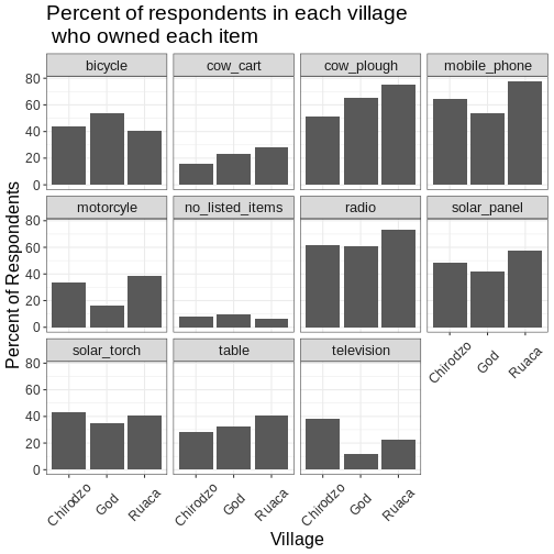
If you like the changes you created better than the default theme, you can save them as an object to be able to easily apply them to other plots you may create. We can also add plot.title = element_text(hjust = 0.5) to centre the title:

R

grey_theme <- theme(axis.text.x = element_text(colour = "grey20", size = 12,
                                               angle = 45, hjust = 0.5,
                                               vjust = 0.5),
                    axis.text.y = element_text(colour = "grey20", size = 12),
                    text = element_text(size = 16),
                    plot.title = element_text(hjust = 0.5))


percent_items %>%
    ggplot(aes(x = village, y = percent)) +
    geom_bar(stat = "identity", position = "dodge") +
    facet_wrap(~ items) +
    labs(title = "Percent of respondents in each village \n who owned each item",
         x = "Village",
         y = "Percent of Respondents") +
    grey_theme

Discussion

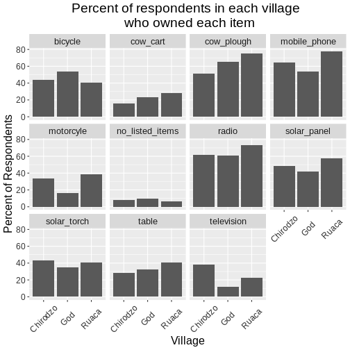
Exercise

With all of this information in hand, please take another five minutes to either improve one of the plots generated in this exercise or create a beautiful graph of your own. Use the RStudio ggplot2 cheat sheet for inspiration. Here are some ideas:

• See if you can make the bars white with black outline.
• Try using a different colour palette (see http://www.cookbook-r.com/Graphs/Colors_(ggplot2)/).

After creating your plot, you can save it to a file in your favourite format. The Export tab in the Plot pane in RStudio will save your plots at low resolution, which will not be accepted by many journals and will not scale well for posters.

Instead, use the ggsave() function, which allows you to easily change the dimension and resolution of your plot by adjusting the appropriate arguments (width, height and dpi).

Make sure you have the fig_output/ folder in your working directory.

R

my_plot <- percent_items %>%
    ggplot(aes(x = village, y = percent)) +
    geom_bar(stat = "identity", position = "dodge") +
    facet_wrap(~ items) +
    labs(title = "Percent of respondents in each village \n who owned each item",
         x = "Village",
         y = "Percent of Respondents") +
    theme_bw() +
    theme(axis.text.x = element_text(color = "grey20", size = 12, angle = 45,
                                     hjust = 0.5, vjust = 0.5),
          axis.text.y = element_text(color = "grey20", size = 12),
          text = element_text(size = 16),
          plot.title = element_text(hjust = 0.5))

ggsave("fig_output/name_of_file.png", my_plot, width = 15, height = 10)

Note: The parameters width and height also determine the font size in the saved plot.

Key Points

• ggplot2 is a flexible and useful tool for creating plots in R.
• The data set and coordinate system can be defined using the ggplot function.
• Additional layers, including geoms, are added using the + operator.
• Boxplots are useful for visualizing the distribution of a continuous variable.
• Barplots are useful for visualizing categorical data.
• Faceting allows you to generate multiple plots based on a categorical variable.

Content from Data Wrangling with tidyr

---

Last updated on 2026-02-24 | Edit this page

Overview

Questions

• How can I reformat a data frame to meet my needs?

Objectives

• Describe the concept of a wide and a long table format and for which purpose those formats are useful.
• Describe the roles of variable names and their associated values when a table is reshaped.
• Reshape a dataframe from long to wide format and back with the pivot_wider and pivot_longer commands from the tidyr package.
• Export a dataframe to a csv file.

dplyr pairs nicely with tidyr which enables you to swiftly convert between different data formats (long vs. wide) for plotting and analysis. To learn more about tidyr after the workshop, you may want to check out this handy data tidying with tidyr cheatsheet.

To make sure everyone will use the same dataset for this lesson, we’ll read again the SAFI dataset that we downloaded earlier.

R

## load the tidyverse
library(tidyverse)
library(here)

interviews <- read_csv(here("data", "SAFI_clean.csv"), na = "NULL")

## inspect the data
interviews

## preview the data
# view(interviews)

Reshaping with pivot_wider() and pivot_longer()

---

There are essentially three rules that define a “tidy” dataset:

1. Each variable has its own column
2. Each observation has its own row
3. Each value must have its own cell

This graphic visually represents the three rules that define a “tidy” dataset:

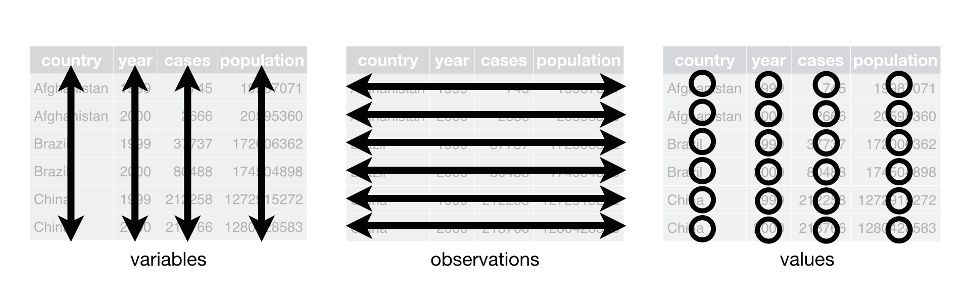R for Data Science, Wickham H and Grolemund G (https://r4ds.had.co.nz/index.html) © Wickham, Grolemund 2017 This image is licenced under Attribution-NonCommercial-NoDerivs 3.0 United States (CC-BY-NC-ND 3.0 US)

In this section we will explore how these rules are linked to the different data formats researchers are often interested in: “wide” and “long”. This tutorial will help you efficiently transform your data shape regardless of original format. First we will explore qualities of the interviews data and how they relate to these different types of data formats.

Long and wide data formats

In the interviews data, each row contains the values of variables associated with each record collected (each interview in the villages). It is stated that the key_ID was “added to provide a unique Id for each observation” and the instanceID “does this as well but it is not as convenient to use.”

Once we have established that key_ID and instanceID are both unique we can use either variable as an identifier corresponding to the 131 interview records.

R

interviews %>% 
  select(key_ID) %>% 
  distinct() %>%
  nrow()

OUTPUT

[1] 131

As seen in the code below, for each interview date in each village no instanceIDs are the same. Thus, this format is what is called a “long” data format, where each observation occupies only one row in the dataframe.

R

interviews %>%
  filter(village == "Chirodzo") %>%
  select(key_ID, village, interview_date, instanceID) %>%
  sample_n(size = 10)

OUTPUT

# A tibble: 10 × 4
   key_ID village  interview_date      instanceID
    <dbl> <chr>    <dttm>              <chr>
 1      8 Chirodzo 2016-11-16 00:00:00 uuid:d6cee930-7be1-4fd9-88c0-82a08f90fb5a
 2     66 Chirodzo 2016-11-16 00:00:00 uuid:a457eab8-971b-4417-a971-2e55b8702816
 3     61 Chirodzo 2016-11-16 00:00:00 uuid:2401cf50-8859-44d9-bd14-1bf9128766f2
 4     60 Chirodzo 2016-11-16 00:00:00 uuid:85465caf-23e4-4283-bb72-a0ef30e30176
 5     34 Chirodzo 2016-11-17 00:00:00 uuid:14c78c45-a7cc-4b2a-b765-17c82b43feb4
 6     65 Chirodzo 2016-11-16 00:00:00 uuid:143f7478-0126-4fbc-86e0-5d324339206b
 7    127 Chirodzo 2016-11-16 00:00:00 uuid:f6d04b41-b539-4e00-868a-0f62b427587d
 8     47 Chirodzo 2016-11-17 00:00:00 uuid:2d0b1936-4f82-4ec3-a3b5-7c3c8cd6cc2b
 9     68 Chirodzo 2016-11-16 00:00:00 uuid:ef04b3eb-b47d-412e-9b09-4f5e08fc66f9
10     37 Chirodzo 2016-11-17 00:00:00 uuid:408c6c93-d723-45ef-8dee-1b1bd3fe20cd

We notice that the layout or format of the interviews data is in a format that adheres to rules 1-3, where

• each column is a variable
• each row is an observation
• each value has its own cell

This is called a “long” data format. But, we notice that each column represents a different variable. In the “longest” data format there would only be three columns, one for the id variable, one for the observed variable, and one for the observed value (of that variable). This data format is quite unsightly and difficult to work with, so you will rarely see it in use.

Alternatively, in a “wide” data format we see modifications to rule 1, where each column no longer represents a single variable. Instead, columns can represent different levels/values of a variable. For instance, in some data you encounter the researchers may have chosen for every survey date to be a different column.

These may sound like dramatically different data layouts, but there are some tools that make transitions between these layouts much simpler than you might think! The gif below shows how these two formats relate to each other, and gives you an idea of how we can use R to shift from one format to the other.

Long and wide dataframe layouts mainly affect readability. You may find that visually you may prefer the “wide” format, since you can see more of the data on the screen. However, all of the R functions we have used thus far expect for your data to be in a “long” data format. This is because the long format is more machine readable and is closer to the formatting of databases.

Questions which warrant different data formats

In interviews, each row contains the values of variables associated with each record (the unit), values such as the village of the respondent, the number of household members, or the type of wall their house had. This format allows for us to make comparisons across individual surveys, but what if we wanted to look at differences in households grouped by different types of items owned?

To facilitate this comparison we would need to create a new table where each row (the unit) was comprised of values of variables associated with items owned (i.e., items_owned). In practical terms this means the values of the items in items_owned (e.g. bicycle, radio, table, etc.) would become the names of column variables and the cells would contain values of TRUE or FALSE, for whether that household had that item.

Once we we’ve created this new table, we can explore the relationship within and between villages. The key point here is that we are still following a tidy data structure, but we have reshaped the data according to the observations of interest.

Alternatively, if the interview dates were spread across multiple columns, and we were interested in visualizing, within each village, how irrigation conflicts have changed over time. This would require for the interview date to be included in a single column rather than spread across multiple columns. Thus, we would need to transform the column names into values of a variable.

We can do both of these transformations with two tidyr functions, pivot_wider() and pivot_longer().

Pivoting wider

---

pivot_wider() takes three principal arguments:

1. the data
2. the names_from column variable whose values will become new column names.
3. the values_from column variable whose values will fill the new column variables.

Further arguments include values_fill which, if set, fills in missing values with the value provided.

Let’s use pivot_wider() to transform interviews to create new columns for each item owned by a household. There are a couple of new concepts in this transformation, so let’s walk through it line by line. First we create a new object (interviews_items_owned) based on the interviews data frame.

R

interviews_items_owned <- interviews %>%

Then we will actually need to make our data frame longer, because we have multiple items in a single cell. We will use a new function, separate_longer_delim(), from the tidyr package to separate the values of items_owned based on the presence of semi-colons (;). The values of this variable were multiple items separated by semi-colons, so this action creates a row for each item listed in a household’s possession. Thus, we end up with a long format version of the dataset, with multiple rows for each respondent. For example, if a respondent has a television and a solar panel, that respondent will now have two rows, one with “television” and the other with “solar panel” in the items_owned column.

R

separate_longer_delim(items_owned, delim = ";") %>%

After this transformation, you may notice that the items_owned column contains NA values. This is because some of the respondents did not own any of the items in the interviewer’s list. We can use the replace_na() function to change these NA values to something more meaningful. The replace_na() function expects for you to give it a list() of columns that you would like to replace the NA values in, and the value that you would like to replace the NAs. This ends up looking like this:

R

replace_na(list(items_owned = "no_listed_items")) %>%

Next, we create a new variable named items_owned_logical, which has one value (TRUE) for every row. This makes sense, since each item in every row was owned by that household. We are constructing this variable so that when we spread the items_owned across multiple columns, we can fill the values of those columns with logical values describing whether the household did (TRUE) or did not (FALSE) own that particular item.

R

mutate(items_owned_logical = TRUE) %>%

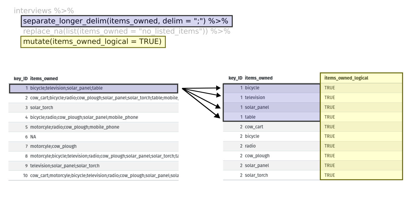
At this point, we can also count the number of items owned by each household, which is equivalent to the number of rows per key_ID. We can do this with a group_by() and mutate() pipeline that works similar to group_by() and summarize() discussed in the previous episode but instead of creating a summary table, we will add another column called number_items. We use the n() function to count the number of rows within each group. However, there is one difficulty we need to take into account, namely those households that did not list any items. These households now have "no_listed_items" under items_owned. We do not want to count this as an item but instead show zero items. We can accomplish this using dplyr’s if_else() function that evaluates a condition and returns one value if true and another if false. Here, if the items_owned column is "no_listed_items", then a 0 is returned, otherwise, the number of rows per group is returned using n().

R

group_by(key_ID) %>% 
  mutate(number_items = if_else(items_owned == "no_listed_items", 0, n())) %>% 

Lastly, we use pivot_wider() to switch from long format to wide format. This creates a new column for each of the unique values in the items_owned column, and fills those columns with the values of items_owned_logical. We also declare that for items that are missing, we want to fill those cells with the value of FALSE instead of NA.

R

pivot_wider(names_from = items_owned,
            values_from = items_owned_logical,
            values_fill = list(items_owned_logical = FALSE))

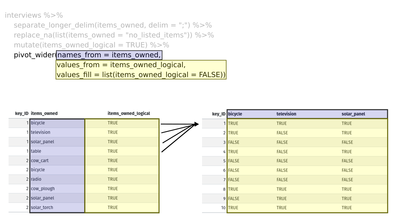
Combining the above steps, the chunk looks like this. Note that two new columns are created within the same mutate() call.

R

interviews_items_owned <- interviews %>%
  separate_longer_delim(items_owned, delim = ";") %>%
  replace_na(list(items_owned = "no_listed_items")) %>%
  group_by(key_ID) %>%
  mutate(items_owned_logical = TRUE,
         number_items = if_else(items_owned == "no_listed_items", 0, n())) %>%
  pivot_wider(names_from = items_owned,
              values_from = items_owned_logical,
              values_fill = list(items_owned_logical = FALSE))

View the interviews_items_owned data frame. It should have r nrow(interviews) rows (the same number of rows you had originally), but extra columns for each item. How many columns were added? Notice that there is no longer a column titled items_owned. This is because there is a default parameter in pivot_wider() that drops the original column. The values that were in that column have now become columns named television, solar_panel, table, etc. You can use dim(interviews) and dim(interviews_wide) to see how the number of columns has changed between the two datasets.

This format of the data allows us to do interesting things, like make a table showing the number of respondents in each village who owned a particular item:

R

interviews_items_owned %>%
  filter(bicycle) %>%
  group_by(village) %>%
  count(bicycle)

OUTPUT

# A tibble: 3 × 3
# Groups:   village [3]
  village  bicycle     n
  <chr>    <lgl>   <int>
1 Chirodzo TRUE       17
2 God      TRUE       23
3 Ruaca    TRUE       20

Or below we calculate the average number of items from the list owned by respondents in each village using the number_items column we created to count the items listed by each household.

R

interviews_items_owned %>%
    group_by(village) %>%
    summarize(mean_items = mean(number_items))

OUTPUT

# A tibble: 3 × 2
  village  mean_items
  <chr>         <dbl>
1 Chirodzo       4.54
2 God            3.98
3 Ruaca          5.57

Challenge

Exercise

We created interviews_items_owned by reshaping the data: first longer and then wider. Replicate this process with the months_lack_food column in the interviews dataframe. Create a new dataframe with columns for each of the months filled with logical vectors (TRUE or FALSE) and a summary column called number_months_lack_food that calculates the number of months each household reported a lack of food.

Note that if the household did not lack food in the previous 12 months, the value input was “none”.

Show me the solution

R

months_lack_food <- interviews %>%
  separate_longer_delim(months_lack_food, delim = ";") %>%
  group_by(key_ID) %>%
  mutate(months_lack_food_logical = TRUE,
         number_months_lack_food = if_else(months_lack_food == "none", 0, n())) %>%
  pivot_wider(names_from = months_lack_food,
              values_from = months_lack_food_logical,
              values_fill = list(months_lack_food_logical = FALSE))

Pivoting longer

---

The opposing situation could occur if we had been provided with data in the form of interviews_wide, where the items owned are column names, but we wish to treat them as values of an items_owned variable instead.

In this situation we are gathering these columns turning them into a pair of new variables. One variable includes the column names as values, and the other variable contains the values in each cell previously associated with the column names. We will do this in two steps to make this process a bit clearer.

pivot_longer() takes four principal arguments:

1. the data
2. cols are the names of the columns we use to fill the a new values variable (or to drop).
3. the names_to column variable we wish to create from the cols provided.
4. the values_to column variable we wish to create and fill with values associated with the cols provided.

R

interviews_long <- interviews_items_owned %>%
  pivot_longer(cols = bicycle:car,
               names_to = "items_owned",
               values_to = "items_owned_logical")

View both interviews_long and interviews_items_owned and compare their structure.

Challenge

Exercise

We created some summary tables on interviews_items_owned using count and summarise. We can create the same tables on interviews_long, but this will require a different process.

Make a table showing the number of respondents in each village who owned a particular item, and include all items. The difference between this format and the wide format is that you can now count all the items using the items_owned variable.

Show me the solution

R

interviews_long %>%
  filter(items_owned_logical) %>% 
  group_by(village) %>% 
  count(items_owned)

OUTPUT

# A tibble: 47 × 3
# Groups:   village [3]
   village  items_owned         n
   <chr>    <chr>           <int>
 1 Chirodzo bicycle            17
 2 Chirodzo computer            2
 3 Chirodzo cow_cart            6
 4 Chirodzo cow_plough         20
 5 Chirodzo electricity         1
 6 Chirodzo fridge              1
 7 Chirodzo lorry               1
 8 Chirodzo mobile_phone       25
 9 Chirodzo motorcyle          13
10 Chirodzo no_listed_items     3
# ℹ 37 more rows

Applying what we learned to clean our data

---

Now we have simultaneously learned about pivot_longer() and pivot_wider(), and fixed a problem in the way our data is structured. In this dataset, we have another column that stores multiple values in a single cell. Some of the cells in the months_lack_food column contain multiple months which, as before, are separated by semi-colons (;).

To create a data frame where each of the columns contain only one value per cell, we can repeat the steps we applied to items_owned and apply them to months_lack_food. Since we will be using this data frame for the next episode, we will call it interviews_plotting.

R

## Plotting data ##
interviews_plotting <- interviews %>%
  ## pivot wider by items_owned
  separate_longer_delim(items_owned, delim = ";") %>%
  replace_na(list(items_owned = "no_listed_items")) %>%
  ## Use of grouped mutate to find number of rows
  group_by(key_ID) %>% 
  mutate(items_owned_logical = TRUE,
         number_items = if_else(items_owned == "no_listed_items", 0, n())) %>% 
  pivot_wider(names_from = items_owned,
              values_from = items_owned_logical,
              values_fill = list(items_owned_logical = FALSE)) %>% 
  ## pivot wider by months_lack_food
  separate_longer_delim(months_lack_food, delim = ";") %>%
  mutate(months_lack_food_logical = TRUE,
         number_months_lack_food = if_else(months_lack_food == "none", 0, n())) %>%
  pivot_wider(names_from = months_lack_food,
              values_from = months_lack_food_logical,
              values_fill = list(months_lack_food_logical = FALSE))

Exporting data

---

Now that you have learned how to use dplyr and tidyr to wrangle your raw data, you may want to export these new datasets to share them with your collaborators or for archival purposes.

Similar to the read_csv() function used for reading CSV files into R, there is a write_csv() function that generates CSV files from data frames.

Before using write_csv(), we are going to create a new folder, data_output, in our working directory that will store this generated dataset. We don’t want to write generated datasets in the same directory as our raw data. It’s good practice to keep them separate. The data folder should only contain the raw, unaltered data, and should be left alone to make sure we don’t delete or modify it. In contrast, our script will generate the contents of the data_output directory, so even if the files it contains are deleted, we can always re-generate them.

In preparation for our next lesson on plotting, we created a version of the dataset where each of the columns includes only one data value. Now we can save this data frame to our data_output directory.

R

write_csv(interviews_plotting, file = "data_output/interviews_plotting.csv")

Key Points

• Use the tidyr package to change the layout of data frames.
• Use pivot_wider() to go from long to wide format.
• Use pivot_longer() to go from wide to long format.