intro to Quarto (Optional)

Last updated on 2026-02-24 | Edit this page

Overview

Questions

What is Quarto?
How can I integrate my R code with text and plots?
How can I convert .qmd files to .html?

Objectives

Create a .qmd document containing R code, text, and plots
Create a YAML header to control output
Understand basic syntax of Quarto and Markdown
Customise code chunks to control formatting
Use code chunks and in-line code to create dynamic, reproducible documents

Quarto

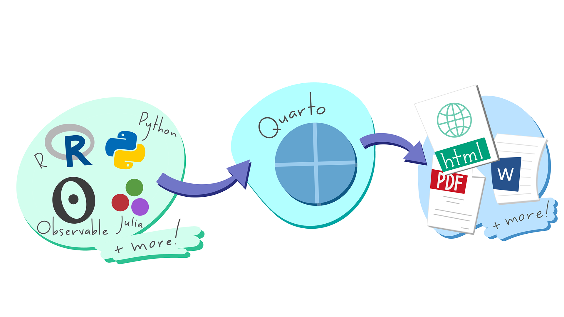
Quarto is a flexible type of document that allows you to seamlessly combine executable R code, and its output, with text in a single document. These documents can be readily converted to multiple static and dynamic output formats, including PDF (.pdf), Word (.docx), and HTML (.html).

The benefit of a well-prepared Quarto document is full reproducibility. This also means that, if you notice a data transcription error, or you are able to add more data to your analysis, you will be able to recompile the report without making any changes in the actual document.

Quarto comes pre-installed with RStudio (as of v2022.07), so no action is necessary.

A schematic representing the multi-language input (e.g. Python, R, Observable, Julia) and multi-format output (e.g. PDF, HTML, Word documents, and more) versatility of Quarto. — A schematic representing the multi-language input **(e.g. Python, R Observable, Julia) and multi-format output (e.g. PDF, HTML, Word documents, and more) versatility of Quarto. Image source: Posit

Creating a Quarto file

To create a new Quarto document in RStudio, click File -> New File -> Quarto Document:

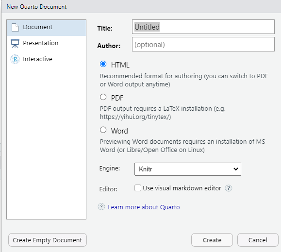
Screenshot of the New Quarto file dialogue box in RStudio

Then click on ‘Create Empty Document’. Normally you could enter the title of your document, your name (Author), and select the type of output, but we will be learning how to start from a blank document.

Basic components of Quarto

To control the output, a YAML (YAML Ain’t Markup Language) header is needed:

---
title: "My Awesome Report"
author: "Emmet Brickowski"
date: ""
format: html
---

The header is defined by the three hyphens at the beginning (---) and the three hyphens at the end (---).

Although not recommended, you can leave the YAML out. Then the output will be by default a HTML file. It’s still better to include the file format in the YAML header by adding the line format: html. You can also adapt the format of the file, to pdf or docx. We will start with an HTML document and discuss the other options later.

You can add more information about your document in the YAML header such as title, date and author. This information will be displayed at the top of your document. There are many more fields that can be added to the YAML header that provide additional information about the document or define the behaviour of the file. But we won’t discuss them now.

After the header, to begin the body of the document, you start typing after the end of the YAML header (i.e. after the second ---).

Markdown syntax

Markdown is a popular markup language that allows you to add formatting elements to text, such as bold, italics, and code. The formatting will not be immediately visible in a markdown (.md) document, like you would see in a Word document. Rather, you add Markdown syntax to the text, which can then be converted to various other files that can translate the Markdown syntax. Markdown is useful because it is lightweight, flexible, and platform independent.

Some platforms provide a real time preview of the formatting, like RStudio’s visual markdown editor (available from version 1.4).

First, let’s create a heading! A # in front of text indicates to Markdown that this text is a heading. Adding more #s make the heading smaller, i.e. one # is a first level heading, two ##s is a second level heading, etc. up to the 6th level heading.

# Title
## Section
### Sub-section
#### Sub-sub section
##### Sub-sub-sub section
###### Sub-sub-sub-sub section

(only use a level if the one above is also in use)

Since we have already defined our title in the YAML header, we will use a section heading to create an Introduction section.

## Introduction

You can make things bold by surrounding the word with double asterisks, **bold**, or double underscores, __bold__; and italicize using single asterisks, *italics*, or single underscores, _italics_.

You can also combine bold and italics to write something really important with triple-asterisks, ***really***, or underscores, ___really___; and, if you’re feeling bold (pun intended), you can also use a combination of asterisks and underscores, **_really_**, **_really_**. You can also use the keyboard shortcuts Ctrl+B for bold and Ctrl+I for italics on Windows and Linux, and Cmd+B for bold and Cmd+I for italics on Mac.

To create code-type font, surround the word with backticks, `code type`.

Now that we’ve learned a couple of things, it might be useful to implement them:

## Introduction

This report uses the **tidyverse** package along with the *SAFI* dataset,
which has columns that include:

Then we can create a list for the variables using -, +, or * keys.

## Introduction

This report uses the **tidyverse** package along with the *SAFI* dataset,
which has columns that include:

- village
- interview_date
- no_members
- years_liv
- respondent_wall_type
- rooms

You can also create an ordered list using numbers:

1. village
2. interview_date
3. no_members
4. years_liv
5. respondent_wall_type
6. rooms

And nested items by tab-indenting:

- village
  + Name of village
- interview_date
  + Date of interview
- no_members
  + How many family members lived in a house
- years_liv
  + How many years respondent has lived in village or neighbouring village
- respondent_wall_type
  + Type of wall of house
- rooms
  + Number of rooms in house

For more Markdown syntax see the following reference guide.

Now we can render the document into HTML by clicking the Render button in the top of the Source pane (top left), or use the keyboard shortcut Ctrl+Shift+K on Windows and Linux, and Cmd+Shift+K on Mac. If you haven’t saved the document yet, you will be prompted to do so when you Render for the first time.

The 'rendering' process: First, **Quarto file is converted to Markdown, which is then converted** (via pandoc) to .html, .pdf, .docx, etc.

Writing a Quarto report

Now we will add some R code from our previous data wrangling and visualisation, which means we need to make sure tidyverse is loaded. It is not enough to load tidyverse** from the console, we will need to load it within our Quarto document**. The same applies to our data. To load these, we will need to create a ‘code chunk’ at the top of our document (below the YAML header).

A code chunk can be inserted by clicking Code > Insert Chunk, or by using the keyboard shortcuts Ctrl+Alt+I on Windows and Linux, and Cmd+Option+I on Mac.

The syntax of a code chunk is:

MARKDOWN

```{r}
#| label: chunk-name
# Here is where you place the R code that you want to run.
```

A Quarto document knows that this text is not part of the report from the ``` that begins and ends the chunk. It also knows that the code inside of the chunk is R code from the r inside of the curly braces ({}). Below the curly braces, you can add code chunk options after the #| sign. In this way, you can for example add a label for the code chunk. Naming a chunk is optional, but recommended. Each chunk label must be unique, and only contain alphanumeric characters and -.

To load tidyverse and our SAFI_clean.csv file, we will insert a chunk and call it ‘setup’. Since we don’t want this code or the output to show in our rendered HTML document, we add an #| include: false option after the curly braces.

MARKDOWN

```{r}
#| label: setup
#| include: false
library(tidyverse)
library(here)
interviews <- read_csv(here("data/SAFI_clean.csv"), na = "NULL")
```

Callout

Important Note!

The file paths you give in a .qmd document, e.g. to load a .csv file, are relative to the .qmd document, not the project root.

As suggested in the Starting with Data episode, we highly recommend the use of the here() function to keep the file paths consistent within your project.

Customising chunk output

We mentioned using include: false in a code chunk to prevent the code and output from printing in the rendered document. There are additional options available to customise how the code-chunks are presented in the output document. The options are entered in the code chunk using the ‘hash pipe’, #|.

Option	Options	Output
`eval`	`TRUE` or `FALSE`	Whether or not the code within the code chunk should be run.
`echo`	`TRUE` or `FALSE`	Choose if you want to show your code chunk in the output document. `echo = TRUE` will show the code chunk.
`include`	`TRUE` or `FALSE`	Choose if the output of a code chunk should be included in the document. `FALSE` means that your code will run, but will not show up in the document.
`warning`	`TRUE` or `FALSE`	Whether or not you want your output document to display potential warning messages produced by your code.
`message`	`TRUE` or `FALSE`	Whether or not you want your output document to display potential messages produced by your code.
`fig-align`	`default`, `left`, `right`, `center`	Where the figure from your R code chunk should be output on the page

Callout

Tip

The default settings for the above chunk options are all true.
The default settings can be modified per chunk, or with knitr::opts_chunk$set(),
Entering knitr::opts_chunk$set(echo = FALSE) will change the default of value of echo to FALSE for every code chunk in the document.

The defaults can also be changed in the YAML header with:

---
knitr:
  opts_chunk:
    echo: false
---

Insert table (self-directed learning)

Next, we will re-create a table from the Data Wrangling episode which shows the average household size grouped by village and memb_assoc. We can do this by creating a new code chunk and calling it ‘interview-tbl’. Or, you can come up with something more creative (just remember to stick to the naming rules).

It isn’t necessary to Render your document every time you want to see the output. Instead you can run the code chunk with the green triangle in the top right corner of the the chunk, or with the keyboard shortcuts: Ctrl+Alt+C on Windows and Linux, or Cmd+Option+C on Mac.

To make sure the table is formatted nicely in our output document, we will need to use the kable() function from the knitr package. The kable() function takes the output of your R code and renders it into a nice looking HTML table. You can also specify different aspects of the table, e.g. the column names, a caption, etc.

Load the data and the tidyverse package in a code chunk with include: false:

Run the code chunk to make sure you get the desired output.

R

interviews %>%
    filter(!is.na(memb_assoc)) %>%
    group_by(village, memb_assoc) %>%
    summarize(mean_no_membrs = mean(no_membrs)) %>%
  knitr::kable(col.names = c("Village", "Member Association", 
                             "Mean Number of Members"))

OUTPUT

`summarise()` has grouped output by 'village'. You can override using the
`.groups` argument.

Village	Member Association	Mean Number of Members
Chirodzo	no	8.062500
Chirodzo	yes	7.818182
God	no	7.133333
God	yes	8.000000
Ruaca	no	7.178571
Ruaca	yes	9.500000

When you are generating a table in quarto the label should be prefixed with tbl-, e.g. tbl-interviews. You can add a caption to the chunk options with tbl-cap: "Your caption here".

MARKDOWN

```{r}
#| label: tbl-interviews
#| tbl-cap: "A useful description about the table."
interviews %>%
    filter(!is.na(memb_assoc)) %>%
    group_by(village, memb_assoc) %>%
    summarize(mean_no_membrs = mean(no_membrs)) %>%
  knitr::kable(col.names = c("Village", "Member Association", 
                             "Mean Number of Members"))
```

OUTPUT

`summarise()` has grouped output by 'village'. You can override using the
`.groups` argument.

A useful description about the table.
Village	Member Association	Mean Number of Members
Chirodzo	no	8.062500
Chirodzo	yes	7.818182
God	no	7.133333
God	yes	8.000000
Ruaca	no	7.178571
Ruaca	yes	9.500000

Many different R packages can be used to generate tables. Some of the more commonly used options are listed in the table below.

Name	Creator(s)	Description
condformat	Oller Moreno (2022)	Apply and visualize conditional formatting to data frames in R. It renders a data frame with cells formatted according to criteria defined by rules, using a tidy evaluation syntax.
DT	Xie et al. (2023)	Data objects in R can be rendered as HTML tables using the JavaScript library ‘DataTables’ (typically via R Markdown or Shiny). The ‘DataTables’ library has been included in this R package.
formattable	Ren and Russell (2021)	Provides functions to create formattable vectors and data frames. ‘Formattable’ vectors are printed with text formatting, and formattable data frames are printed with multiple types of formatting in HTML to improve the readability of data presented in tabular form rendered on web pages.
flextable	Gohel and Skintzos (2023)	Use a grammar for creating and customizing pretty tables. The following formats are supported: ‘HTML’, ‘PDF’, ‘RTF’, ‘Microsoft Word’, ‘Microsoft PowerPoint’ and R ‘Grid Graphics’. ‘R Markdown’, ‘Quarto’, and the package ‘officer’ can be used to produce the result files.
gt	Iannone et al. (2022)	Build display tables from tabular data with an easy-to-use set of functions. With its progressive approach, we can construct display tables with cohesive table parts. Table values can be formatted using any of the included formatting functions.
huxtable	Hugh-Jones (2022)	Creates styled tables for data presentation. Export to HTML, LaTeX, RTF, ‘Word’, ‘Excel’, and ‘PowerPoint’. Simple, modern interface to manipulate borders, size, position, captions, colours, text styles and number formatting.
pander	Daróczi and Tsegelskyi (2022)	Contains some functions catching all messages, ‘stdout’ and other useful information while evaluating R code and other helpers to return user specified text elements (e.g., header, paragraph, table, image, lists etc.) in ‘pandoc’ markdown or several types of R objects similarly automatically transformed to markdown format.
pixiedust	Nutter and Kretch (2021)	‘pixiedust’ provides tidy data frames with a programming interface intended to be similar to ’ggplot2’s system of layers with fine-tuned control over each cell of the table.
reactable	Lin et al. (2023)	Interactive data tables for R, based on the ‘React Table’ JavaScript library. Provides an HTML widget that can be used in ‘R Markdown’ or ‘Quarto’ documents, ‘Shiny’ applications, or viewed from an R console.
rhandsontable	Owen et al. (2021)	An R interface to the ‘Handsontable’ JavaScript library, which is a minimalist Excel-like data grid editor.
stargazer	Hlavac (2022)	Produces LaTeX code, HTML/CSS code and ASCII text for well-formatted tables that hold regression analysis results from several models side-by-side, as well as summary statistics.
tables	Murdoch (2022)	Computes and displays complex tables of summary statistics. Output may be in LaTeX, HTML, plain text, or an R matrix for further processing.
tangram	Garbett et al. (2023)	Provides an extensible formula system to quickly and easily create production quality tables. The processing steps are a formula parser, statistical content generation from data defined by a formula, and rendering into a table.
xtable	Dahl et al. (2019)	Coerce data to LaTeX and HTML tables.
ztable	Moon (2021)	Makes zebra-striped tables (tables with alternating row colors) in LaTeX and HTML formats easily from a data.frame, matrix, lm, aov, anova, glm, coxph, nls, fitdistr, mytable and cbind.mytable objects.

Challenge

Exercise

Play around with the different options in the chunk with the code for the table, and re-Render to see what each option does to the output.

What happens if you use eval: false and echo: false? What is the difference between this and include: false?

Solution to Exercise

Create a chunk with eval: false, echo: false, then create another chunk with include: false to compare. eval: false and echo: false will neither run the code in the chunk, nor show the code in the rendered document. The code chunk essentially doesn’t exist in the rendered document as it was never run. Whereas include: false will run the code and store the output for later use.

In-line R code (self-directed learning)

Now we will use some in-line R code to present some descriptive statistics. To use in-line R-code, we use the same backticks that we used in the Markdown section, with an r to specify that we are generating R-code. The difference between in-line code and a code chunk is the number of backticks. In-line R code uses one backtick (r), whereas code chunks use three backticks (r).

For example, today’s date is `r Sys.Date()`, will be rendered as: today’s date is 2026-02-24.
The code will display today’s date in the output document (well, technically the date the document was last rendered).

The best way to use in-line R code, is to minimise the amount of code you need to produce the in-line output by preparing the output in code chunks. Let’s say we’re interested in presenting the average household size in a village.

R

# create a summary data frame with the mean household size by village
mean_household <- interviews %>%
    group_by(village) %>%
    summarize(mean_no_membrs = mean(no_membrs))

# and select the village we want to use
mean_chirodzo <- mean_household %>%
  filter(village == "Chirodzo")

Now we can make an informative statement on the means of each village, and include the mean values as in-line R-code. For example:

The average household size in the village of Chirodzo is `r round(mean_chirodzo$mean_no_membrs, 2)`

becomes…

The average household size in the village of Chirodzo is 7.08.

Because we are using in-line R code instead of the actual values, we have created a dynamic document that will automatically update if we make changes to the dataset and/or code chunks.

Plots (self-directed learning)

Finally, we will also include a plot, so our document is a little more colourful and a little less boring. We will use the interview_plotting data from the previous episode.

If you were unable to complete the previous lesson or did not save the data, then you can create it in a new code chunk.

R

## Not run, but can be used to load in data from previous lesson!
interviews_plotting <- interviews %>%
  ## pivot wider by items_owned
  separate_rows(items_owned, sep = ";") %>%
  ## if there were no items listed, changing NA to no_listed_items
  replace_na(list(items_owned = "no_listed_items")) %>%
  mutate(items_owned_logical = TRUE) %>%
  pivot_wider(names_from = items_owned, 
              values_from = items_owned_logical, 
              values_fill = list(items_owned_logical = FALSE)) %>%
  ## pivot wider by months_lack_food
  separate_rows(months_lack_food, sep = ";") %>%
  mutate(months_lack_food_logical = TRUE) %>%
  pivot_wider(names_from = months_lack_food, 
              values_from = months_lack_food_logical, 
              values_fill = list(months_lack_food_logical = FALSE)) %>%
  ## add some summary columns
  mutate(number_months_lack_food = rowSums(select(., Jan:May))) %>%
  mutate(number_items = rowSums(select(., bicycle:car)))

Plots created in Quarto should have a label prefixed with fig-, e.g. #| label: fig-fancy-plot.

Challenge

Exercise

Create a new code chunk for the plot, and copy the code from any of the plots we created in the previous episode to produce a plot in the chunk. I recommend one of the colourful plots.

If you are feeling adventurous, you can also create a new plot with the interviews_plotting data frame.

Solution to Exercise

MARKDOWN

```{r}
#| label: fig-fancy-plot
#| answer: true
#| purl: false
interviews_plotting %>%
  ggplot(aes(x = respondent_wall_type)) +
  geom_bar(aes(fill = village))
```

We can also create a caption with the chunk option fig-cap: "Caption here", and add some nicer labels using the labs() function.

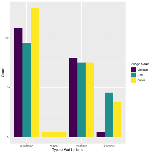
MARKDOWN

```{r}
#| label: fig-chunk-name
#| fig-cap: "I made this plot while attending an awesome Data Carpentries workshop where I learned a ton of cool stuff!"
#| echo: false

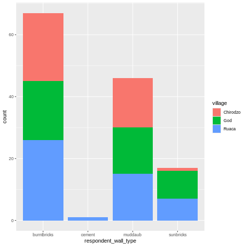
interviews_plotting %>%
  ggplot(aes(x = respondent_wall_type)) +
  geom_bar(aes(fill = village), position = "dodge") + 
  labs(x = "Type of Wall in Home", y = "Count", fill = "Village Name") +
  scale_fill_viridis_d() # add colour deficient friendly palette
```

I made this plot while attending an awesome Data Carpentries workshop where I learned a ton of cool stuff!

…or, ideally, something more informative.

Now, you may have been wondering why I insisted that you prefix the labels of your tables in figures, but there is a useful reason for this! It allows you to cross-reference them in the text of your document, and it requires that the label is unique, and that they have the correct prefix.

For example, we can talk about the table we made earlier and reference it using the label @tbl-interview, which, when rendered, becomes Table 1.

We can do the same with our figures. For example, @fig-fancy-plot becomes Figure 1. The number will of course depend on whether any plots or figures comes before it, but since you just need to reference the label, there’s no need to know what number a specific plot has in a document (especially useful for figure-heavy documents).

Other output options (self-directed learning)

You can convert Quarto to a PDF or a Word document (among others). Put pdf or word in the initial header of the file to indicate the desired output format.

---
format: word
---

Callout

Note: Creating PDF documents

Creating .pdf documents may require installation of some extra software. The R package tinytex provides some tools to help make this process easier for R users. With tinytex installed, run tinytex::install_tinytex() to install the required software (you’ll only need to do this once) and then when you render to pdf tinytex will automatically detect and install any additional LaTeX packages that are needed to produce the pdf document. Visit the tinytex website for more information.

Callout

Note: Inserting citations into a Quarto file

It is possible to insert citations into a Quarto file using the editor toolbar. The editor toolbar includes commonly seen formatting buttons generally seen in text editors (e.g., bold and italic buttons). The toolbar is accessible by using the settings dropdown menu (next to the ‘Render’ dropdown menu) to select ‘Use Visual Editor’, also accessible through the shortcut ‘Crtl+Shift+F4’. From here, clicking ‘Insert’ allows ‘Citation’ to be selected (shortcut: ‘Crtl+Shift+F8’). For example, searching ‘10.1007/978-3-319-24277-4’ in ‘From DOI’ and inserting will provide the citation for ggplot2 [@wickham2016]. This will also save the citation(s) in ‘references.bib’ in the current working directory.

Visit the R Studio website for more information. Tip: obtaining citation information from relevant packages can be done by using citation("package").

Resources

Markdown tutorial
Official Quarto website (comprehensive resource of tutorials and documentation)
Welcome to Quarto - workshop by Posit (former RStudio)
R Markdown: The Definitive Guide - book by the RStudio team on R Markdown, the predecessor of Quarto

Key Points

Quarto is useful for creating reproducible documents combining text and executable R code.
Specify chunk options to control formatting of the output document